
There are a plethora of tutorials on how to identify and count unique values on the Excel work file. If you have read any of them, then you should know how to identify unique or distinct values in Excel. This is achieved in just three steps – identification, filtrating, and copying of the unique values. However, most of these methods are very cumbersome. But I will guide you through how to find and filter out unique values on the Excel column using special formulas and other quick methods.
How to get unique values in Excel
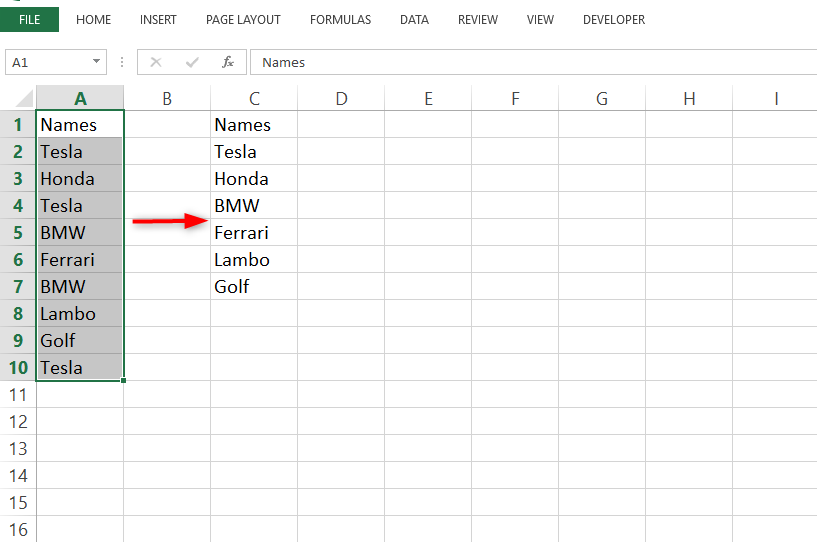
Before we zoom into the tutorial, it is Paramount that we familiarize ourselves with the meaning of unique values in Excel. In Excel, unique values are values that do not repeat. They are mentioned once in the list. Take a look at the image below to catch a glimpse of unique values.
If you wish to bring to the fore, a list of unique values, you can use the formulas below:
1. The Array formula:
=IFERROR(INDEX($A$2:$A$10, MATCH(0, COUNTIF($B$1:B1,$A$2:$A$10) + (COUNTIF($A$2:$A$10, $A$2:$A$10)<>1), 0)), ""
>> The array formula is executed by pressing "Ctrl + Shift + Enter"
2. The regular formula:
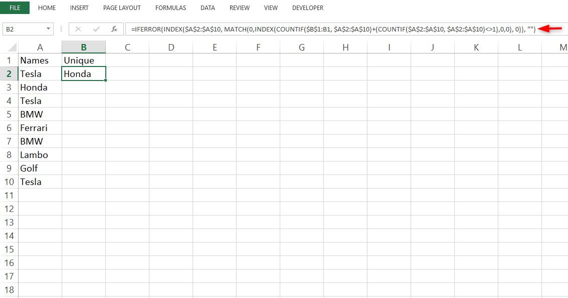
=IFERROR(INDEX($A$2:$A$10, MATCH(0,INDEX(COUNTIF($B$1:B1, $A$2:$A$10)+(COUNTIF($A$2:$A$10, $A$2:$A$10)<>1),0,0), 0)), "")
>> You will execute the regular formula when you press "Enter."
In the above formulas, the following references are used:
- A2: A10 is the source list
- B1 is the cell at the top of the unique list. Here, we begin the unique list from B2 and include B1 to the formula as stated – (B2-1=B1)
- Now, in your own case, the unique list may start from cell C3. In such a case, change from $B$1:B1 to $C$2:C2.
Here, our emphasis is on A2: A20 and we can use the formula to extract unique values from the Excel sheet as follows:
1. Pick one of the formulas and tweak it in line with your data.
2. After tweaking the formula, locate the first cell and enter the formula. In this example, it's B2.
3. Drag the fill handle to copy the formula down. Drag as far as you want.
4. The unique values are embedded in the IFERROR, so you have the liberty to copy the formula down till you reach the end of the table. There are no issues with the number of unique values that you extract. Your data will not clutter with errors if the unique values are few.
Using the Advanced Filter
If you are not conversant with formulas, you can quickly select the unique values by using the advanced filter on Excel. We do so by following the steps below:
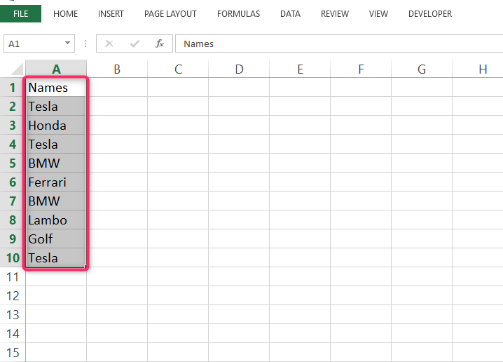
1. Firstly, locate and select the column from which where you want to extract data from.
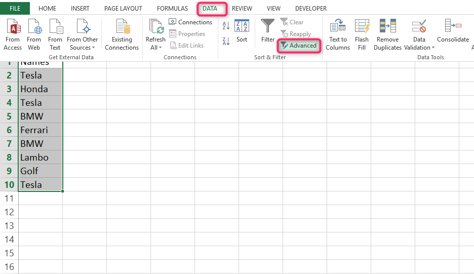
2. Navigate to the Data tab.
3. Proceed by clicking "Sort and filter group''. Go ahead and click the advanced button.
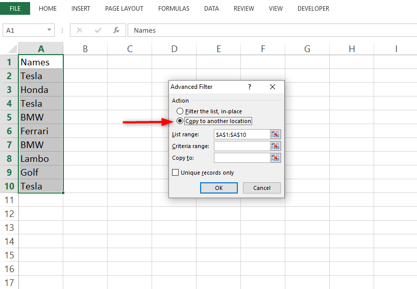
4. After the advanced filter has opened, click the "Copy to another location" radio button.
5. Check the list named "Range box,'' and complete the verification process to attest that the range is correct.
6. Identify the box – "copy to", and the range of the destination. Enter in the topmost cell.
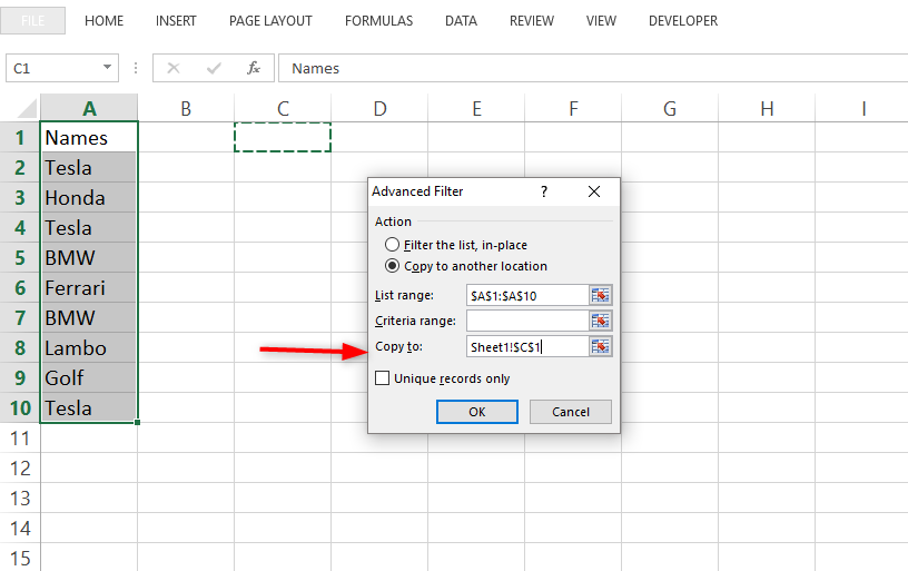
7. After filtering your data, It's only the active sheet that you can copy to.
8. Identify all the unique values and select.
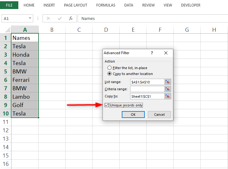
9. Now, open the options for advance filter and configure accordingly.
Lastly, select, Ok, and your result will display.