
Each time you create data in any of the files and tools that can hold data; you always have the free will to manipulate or shape your data the way you want. You can filter, you can color, you can change the font and even to rotation to any degree you like.
The process or the act of turning objects or items around the axis or the center is what we call rotation. Rotation can occur at any degree you want it to. Although in excel sheets you can only rotate from -90 to 90 degrees.
In most cases, we rotate data to change its original appearance to a newer format or display. Rotation also is done to rectify the mistake done while typing, maybe the content is anti-clockwise and it is unreadable.
To do a data rotation, there is a couple of steps involved and which are discussed below in detail.
Step 1
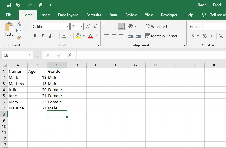
Record some data in a new excel sheet. This will be the first step to approach if we are to rotate data in an excel sheet. The data is just general and of your choice. Take a look at the sample below.
Step 2
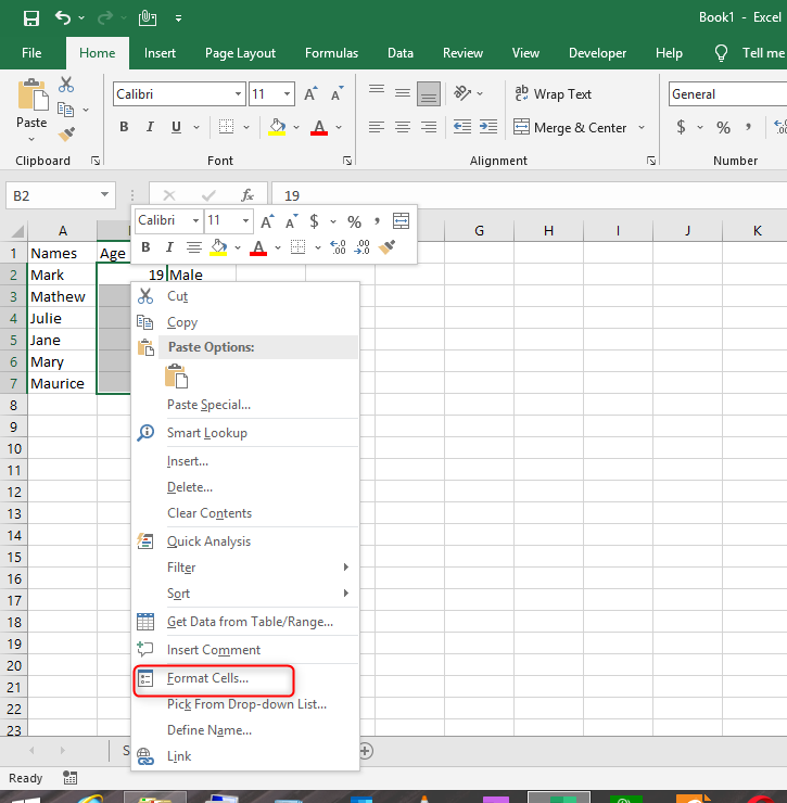
The second step is now to start rotation of the data in the cell we want it rotated. Now on your excel sheet, select or highlight the column or the row you would like to rotate. After highlighting, right-click on your mouse. A window of options will appear on the right-hand side of your selected data. Scroll down and click on format cells.
Step 3
Upon clicking on the format cells option another window will appear where you can select the degrees to rotate your data.
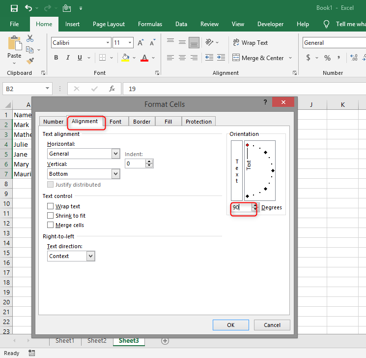
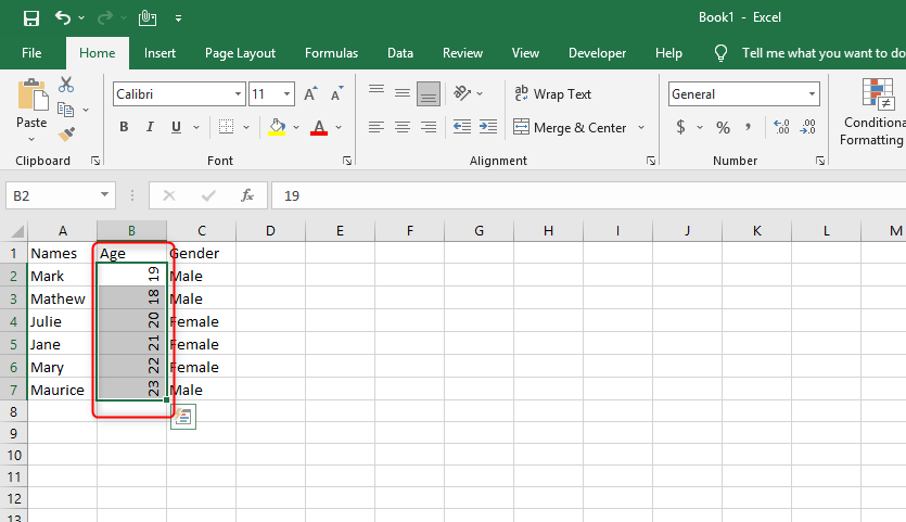
Increment the value of degrees to 90 because it is the value we need the data rotated to. Click on ok to make the changes. You will realize the middle column in the excel sheet will be rotated to 90 degrees and the data contained in the column will be displayed vertically as in the case shown below.