
In excel we have numerous built-in functions, commands, formulas, and even capabilities. All these built-in functions have a particular role to play in the excel sheets. Their functions may differ depending on their general usage in the excel sheets.
We do can the sum of columns or rows in excel sheets with the aid of built-in formulas. These columns or rows can either be filtered or unfiltered. Filtering is the act or process of separating particular objects or rows from others based on their differences.
To do the sum of a filtered column is the process or activity of adding all the visible or the filtered columns in a given data set in an excel sheet. We do this with the aid of the sum formula. Below are some of the steps to find the sum of filtered columns in a given excel sheet together with the samples.
Steps to filter data in a Column in Excel
Step 1
From your laptop or computer, insert or record some general data into a new or a blank excel sheet like the one shown below.

Step 2
The second step is to filter the values we need them to remain visible to find their sum.
- To have this done, Select the marks' column and under the Home tab,

- click on sort and filter.
- Under the sort and filter command select on the filter.

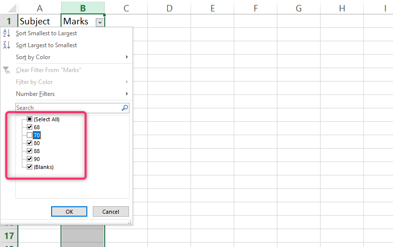
- The marks' column will appear to have a drop-down filter arrow as shown below in the image.

Step 3
Having done the first steps of filtering on step two, select the drop-down arrow on the marks' column and scroll down. Mark the values you intend to filter and click on ok to make the changes.
Steps to sum filtered data in Excel
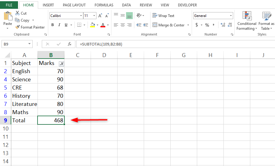
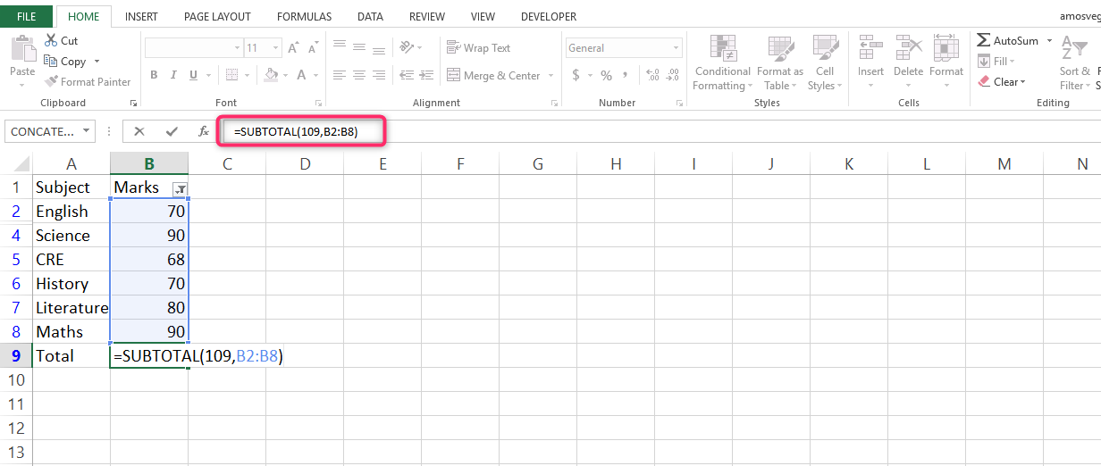
- The final step is now to get the sum of the filtered columns. We do this with the help of the function SUBTOTAL.
- In the formula bar from our excel sheet enter the formula, =SUBTOTAL (109, B2: B8),
- click on the enter button to execute the command. The result will appear on cell B8 which is our result cell.