
Excel is a popular spreadsheet program for financial analysis. Over the years, Excel has served many individuals and organizations in the area of financial modeling. It is embedded with tons of functions and formulas that one can easily use for financial analysts.
Here in this article, we shall highlight the top 10 Excel formulas that you can use for financial operations.
1. Net Present Value (XNPV)
NPV, the Net Present Value is a financial operation that measures profit within a given period of time. The NPV measures the differences between the present amount of cash that flows in and the present amount of cash that flows out within a certain period.
XNPV keeps account of specific dates and is very efficient in analyzing the flow of cash.
The Syntax for the XNPV function is:
=XNPV(rate, values, dates)

2. The function value (FV)
The Function value computes the future value of an asset and the amount of money to expect in due course. It assumes the rate of future growth by drawing the premise from the current value of the asset and regular income.
The Syntax for FV function is
= FV(rate, nper, pmt, [pv], [type])
N/B: The Argument, "type" is used conditionally. It is applied when payment is due at the beginning of the period but is omitted if payment is due at the end.

3. Internal Rate of Return (XIRR)
Financial analysts can use the XIRR to compute the rates of profit returns for a series of dates. It estimates the potential rates of profit that can accrue on future investments. It is not influenced by factors outside the company, such as the cost of capital and inflation.
To calculate the internal rate of return for varying dates of cash flows, use the XIRR function.
The Syntax for deducing XIRR function is:
= XIRR(values, dates, [guess])
N/B: The Argument, "guess" is an optional number that you decide to choose considering if it is close to the result or not. Use 10% in cases where you decide to omit it.

4. Modified internal rate of return (MIRR)
Financial analysts use the MIRR extensively when working with several investments of equal value and for the planning of capital budgets. It operates with the assumption that the asset will yield profits. It considers the amount expended in setting up the investment as well as the interest accrued from the reinvestment.
The Syntax for deducing MIRR:
= MIRR(values, finance_rate, reinvest_rate)

5. PMT
PMT is the value of money required within a given timeframe for the payment of an asset. It comes with a steady interest rate.
Here is the Syntax for evaluating PMT:
PMT = (Rate, Nper, PV, [FV], [Type])
Rate = is the value for the interest rate per period.
Nper = is the number of periods
PV = stands for the present value
[FV] = Denotes the potential value of a loan. Use zero in cases where it is not mentioned
[Type] = is used to denote that payment will be made at the beginning. It is assumed that payment is made at the end of the period when it is not mentioned.

6. NPER
Loans are paid off within a certain number of periods. You can use NPER to deduce the number of periods required in paying off the loan.
The Syntax for NPER on Excel:
NPER = (Rate, PMT, PV, [FV], [Type])
Rate = is the value of interest accrued per period
PMT = the value of money required within a given timeframe for the payment of an asset.
PV = stands for the present value.
[FV] = Denotes the potential value of a loan. Use zero in cases where it is not mentioned
[Type] = is used to denote that payment will be made at the beginning. It is assumed that payment is made at the end of the period when it is not mentioned.

7. RATE
There is always a specific amount of interest required to pay off a loan completely. We can be using the RATE function on Excel to estimate the interest rate accrued within the specified time.
Syntax for RATE
RATE = (NPER, PMT, PV, [FV], [Type], [Guess])
Nper = number of periods
PMT = the value of money required within a given timeframe for the payment of an asset.
PV = stands for the present value.
[FV] = Denotes the potential value of a loan. Use zero in cases where it is not mentioned
[Type] = is used to denote that payment will be made at the beginning. It is assumed that payment is made at the end of the period when it is not mentioned.
[Guess] = is your assumed value for RATE

8. Effect
Analysts use this function to calculate to estimate the effective interest rate for the year. The interest rate accrues from the period required as well as the nominal interest rate that it supplies.
The Syntax for Effect is:
EFFECT = (Nominal_Rate, NPERY)
Nominal_Rate is the Nominal Interest Rate
NPERY is the number of yearly compounding

9. NOMINAL
The Nominal yearly rate is calculated after deducing the number of periods and the effective annual rate. In this case, the number of periods is compounded yearly.
Excel syntax for Nominal is:
NOMINAL = (Effect_Rate, NPERY)
Effect_Rate = the effective interest rate for the year
NPERY = Yearly number of compounding

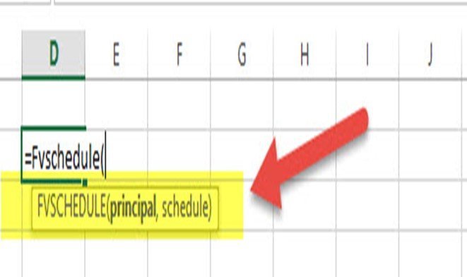
10. FVSCHEDULE:
This is very useful in calculations involving a varying interest rate. You can use it to estimate future value.
Excel syntax for FVSCHEDULE is:
FVSCHEDULE = (Principal, Schedule)
Principal = is the current cost of the asset.
Schedule = a well-defined collection of interest rates. When working on Excel, we select the range and also make use of varying boxes.
Virtually all the formulas are inbuilt, and they are very simple to use too.
Additional Information: 10 Top Excel Financial Functions
The following are extra functions in Excel.
1. IPMT
The IPMT function works well when combined with the PMT formula. It calculates the interest portion for fixed debt payments. When using this combination, you can easily separate the interest payment in each period and get the principal in each period by determining the difference between PMT and IPMT. Its generic formula is:
= IPMT(rate, current period #, total # of periods, present value)
Example:
You can calculate the interest payment in the fifth year on a 30-year loan with an interest rate of 4.5%, with the current value of $10,000 as shown below:
=IPMT(C6,C7,C8,C5)

2. DB
Accountants and financial professionals can benefit from the DB function greatly, especially if they want to evade accumulating a large Declining Balance (DB) depreciation schedule. That is because can easily calculate the depreciation expense in each period. Its generic formula is:
=DB(cost, salvage value, life/# of periods, current period)

3. SLOPE
The SLOPE function is also an essential formula for finance professionals to want to calculate the Beta (volatility) of stock when evaluating analysis and financial modeling. Although such professionals can easily get the stock's Beta from Bloomberg and CapIQ, sometimes it is wise to create a formula for safer and quicker financial analysis. Hence, the formula calculates the stock’s Beta based on your preferred index and the weekly returns. Its syntax is:
=SLOPE(dependent variable, independent variable)

4. The Present Value (PV)
The present value (PV) function is easier to apply if you already know about the future value (FV) function. Its syntax is:
= PV(Rate, Nper, [Pmt], FV, [Type]), where;
Rate is the interest charged per period.
Nper is the number of periods.
[Pmt] is the payment per period.
FV is the future value.
[Type] is used if payment is made. If no payment was made or mentioned, you assume the payment was made at the end of the period.
Example:
If you have the future value of an investment where the payment is made annually with an interest of 10%, you can calculate the present value as follows:
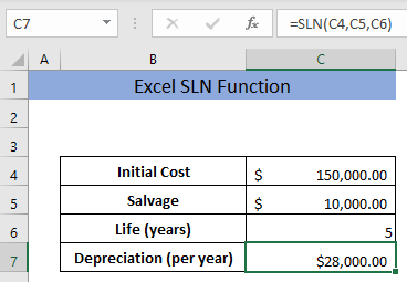
5. SLN
The SLN function calculates the depreciation using a straight-line method. Its syntax is:
= SLN(Cost, Salvage, Life), where;
cost is the value of an asset when buying (its initial price).
salvage is the value of an asset after depreciation.
life is the period over which the asset has depreciated.
Example:
You can calculate the depreciation charged on a machinery per year for 10 years based on its initial cost and salvage value as follows:
6. PPMT
The PPMT function calculates the principal payment for a loan based on periodic constant installments and interest rates. Its syntax is:
= PPMT(Rate, Per, Nper, PV, [FV],[Type]), where;
Rate is the interest rate charged on the loan.
Per is the specific period recorded between 1 and NPER.
Nper is the total number of installments or periods.
PV is the present value of the loan.
FV is the future value of the loan after the last payment.
Type is a logic value. You can enter 1 if the payment is made at the start of the period or 0 if the payment is made at the end of the period. Alternatively, you can leave it blank and Excel will count it as 0.
Example:
You can calculate the principal payment for each year for a 4-year loan with an interest rate of 7% p.a as follows:
