Excel offers a lot of powerful features to use while working with spreadsheets. Pivot tables are among them. A pivot table allows the user to group large data sets accordingly. Using a pivot table allows you to summarize data in a clear and precise manner. The table is always in a summarized tabular format which makes it easier for data reporting and analysis. These tables are useful when you have long rows or columns of data that appear to be jumbled up. It stems from the fact that you can pivot (rotate) the table's data for you to view it from a different perspective. Keep in mind that this does not mean the original data is changed or deleted, but it is reorganized for a data reader to extract useful information.
Due to these features that entail a pivot table, some users find it hard to construct one, which is not the case as the procedure is straightforward. Let's look at how to create a pivot table in excel from the article below.
Steps to follow
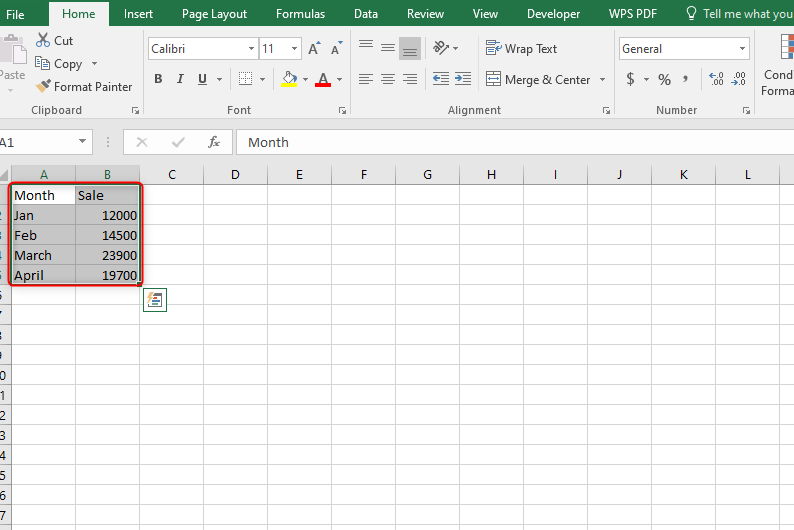
1. Launch the Microsoft Excel program. Open the Excel spreadsheet you want to create the pivot table in or open the worksheet that contains the table you want to summarize. Select any cell in the table.
To be successful, you have to ensure that your table has no blanks and each column has a title head.

2. From the main menu ribbon, access the Insert tab. On the Tables group, select PivotTable. Doing this, Excel will open a dialogue box.

3. Select the data you want to use.

By default, Excel will select all the data in your active worksheet. Click and drag your cursor to choose the specific data you need from the spreadsheet. If not, type the cell range manually in the table/Range field.
In case you are using external data, select the 'Use an external data source' option and click 'Choose Connection,' which will enable you to browse for the data file you want.

4. Select the pivot's table location

From the still open dialogue box, choose your pivot's table location. It can either be a new worksheet or an existing one. We do this because, by default, Excel will create the table in a new worksheet.
5. Click OK.
Excel adds a blank grid for the new pivot table. The PivotTable Field List task pane also appears. Select the desired fields from the 'Choose fields to add to report' area. Drag and drop a field name from this area to add to the Report list box. The report list box contains four boxes: Report Filter, Column Labels, Row Labels, and Values.

6. Continue to move and manipulate your data. To achieve this, drag and drop your data until you get the desired results.
Conclusion
A pivot table enables a user to create and analyze large data sets in Excel worksheets. With the above steps, you can create your pivot tables without the prejudices of the process being hard or complicated.
