Excel takes the lead when it comes to automation operations on cells. I personally love Excel due to its robustness in offering various functionalities to the user. Users can, therefore, manipulate their own data the way they like or wish without any restrictions. Generation of serial numbers is one of the things that I find adventurous in excel. Serial numbers can thus be assigned automatically to a specified column using a formula in a matter of a click of few keys and a lovely drag of cells. This article is therefore purposely aimed at illustrating a simple formula for generating serial numbers. Windows 8 has been used as the Operational Operating system but many similarities are present with higher versions so don't feel left out if you are using a lower or higher version. To create unique sequential numbers please follow the following steps:
Procedure for generating unique Sequential Numbers:
Step 1: For those using windows operating system, press the Windows button or use your mouse to click the start button.
This displays a list of programs that are installed on your computer. If you have installed only one version of MS office say MS OFFICE 2010 then MS excel 2010 should be among the applications listed.
In most cases, a search pane is also visible when the windows or start button is pressed or clicked. The search pane enables users to perform a search operation instead of manually searching through the list of listed programs.

Step 2: Search for the word by typing the word "EXCEL" in the search bar or pane and choose the icon for MS excel.
The more you type in the search bar the word excel, the more the option becomes prioritized according to the criteria of the search name. For those using windows 8
make sure that the search selection is on the app's search option to display applications.
From the list of application try to find the excel version that holds your excel work for those who may have different versions of MS office.
Step 3: Click on the excel icon. It should have a corresponding name for example: "Microsoft excel [year]" and wait for it to load. The excel icon is usually checked with a dominant green color.
Step 4: Navigate to the File tab button of excel ribbon and click recently for those using MS word 2010 and higher versions.

Select your excel work of choice by clicking on it. You can also use the open option in other versions.
Step 5: Your Excel document will be loaded.

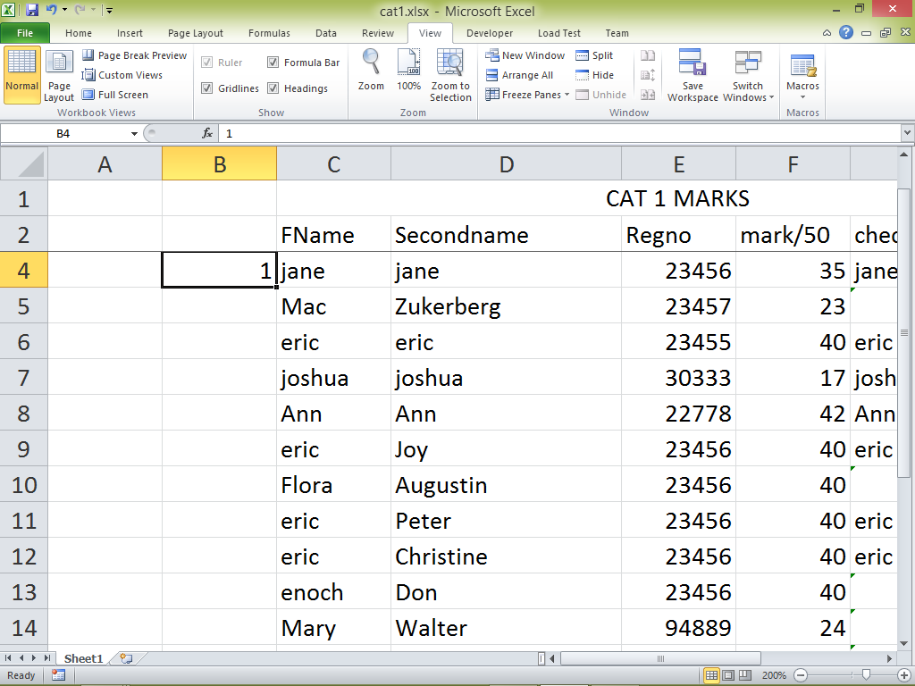
Step 6: Ensure that you have an empty column towards the leftmost side of cells. If not; insert an empty column.
In my case, there is an empty column B but I will add another empty column for illustration purposes.
Step 7: To insert a column say an empty column C do the following:
Move the cursor to the topmost column headers and ensure that the cursor is between the column boundaries as below.

Step 8: Right-click while the cursor is at the boundary and selects "Insert"

Step 9: A new column shall be inserted as below:

Step 10: At the cell, C2 Add a label named serial to act as column header as follows.

Step 11: Move the active cell pointer to C3.

You will note that the first two rows are at freeze state for my worksheet. To freeze the rows in yours please do the following:
I) highlight the top 3 rows.
II) Click the View tab on the excel ribbon.
III) Select the freeze panes options.
(IV) You can now scroll with the first two rows being on freeze state. This means that they don't move when scrolling all through.
Step 12: Enter the formula below in cell C3.
=IF
(F3="","",SUBTOTAL(3,$F$3:F3))

Explanation of formula
IF function is used to set the condition in the formula. The first " " checks whether F3 is empty while the second " " sets the value of c3 to empty if registration no is missing. This means no value is displayed if a Registration no is missing. Note that in the formula we have used F3 as the reference since it contains unique values, which are registration numbers that at no case are expected to ever be blank for any complete record.
The formula can be entered either in the formula bar or while inside the cell. In my case, I have typed the formula in the formula bar while the curse laid to rest on cell C3.
Step 13: Now press enter key. This executes the formula you have typed in the formula bar.
Step 14: You will get the output below

Step 15: Now drag the bottom right corner throughout the column.
The column will automatically recalculate the serial numbers. The serial numbers will be sequential with each serial number being the previous one plus one.
