Whenever we are handling numbers, values, ranges, and figures there is always the need to identify the minimum value of all the values and the maximum values of all the values. We get the minimum or maximum values in any given set of data to be able to find the range of the data.
In an excel sheet when we record data, we also have the urgency to get its minimum and its maximum with this you can find the mean, mode, and median of the data set. You can find the range of the data you just recorded, for example, is it relying on the great side or the small side secondly is it occurring mostly at the minimum or the maximum.
For us to calculate the minimum and maximum values in any given excel sheet there are several steps that we can follow to achieve the correct result. These steps are discussed below in detail.
You can use MIN and MAX in the same formula if you want to convert the lowest or the highest value to the minimum or maximum
Steps to use MIN and MAX in the same formula
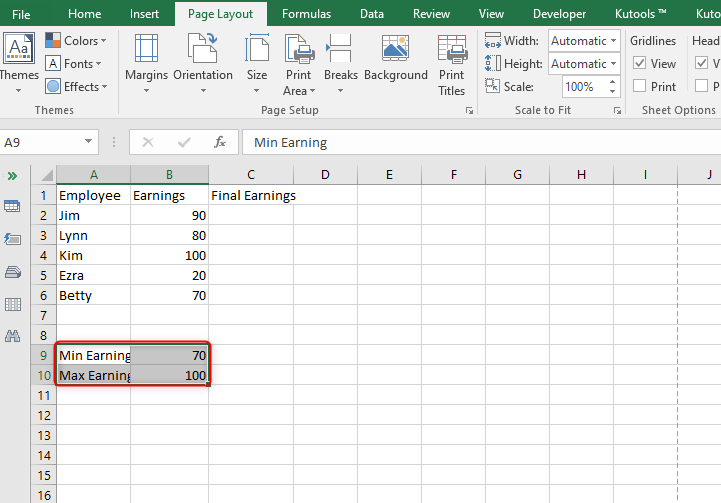
1. Let's take the following data as an example. We want to make sure that every employee earns $70 and above regardless of their sales. So we can use the MIN MAX to regulate the earnings.

2. Create reference cells for MIN and MAX earnings.

3. Now let us regulate the earnings to a minimum of 70 and a maximum of 100. Enter the following formula in cell C5 =MAX(MIN(B2,$B$11),$B$10)

4. Now drag the formula to the rest of the cells. As you can see in the picture below the earnings have been converted from 20 to 70 automatically using the MIN and MAX functions in the same formula

How to use MIN and Max formula Separately
Step 1
To get the maximum and minimum values, you need to come up with a data set containing values in numeric form. Open a blank excel sheet and record your data in it. For example, you can use one column for job code and the other column for salary.

Step 2
Now that the excel sheet has been created, we are now going to get the minimum and maximum values from the data we have. To do this, there are a couple of formulas involved. To find the value of the minimum figure we are going to use =MIN (B2: B6). This formula will output the smallest value of all in the data set above.

To find the maximum value in the data above, we are going to use the formula =MAX (b2: B6). Again this formula will display the largest value of all in the data set above.

MINIFS Function
MINIFS function is usually used to determine the smallest number according to one or many criteria. Arguments associated with the MINIFS formula:
- Min_ range: Is the range where you will find the smallest value.
- Range1: The first range to look for in a criterion.
- Criteria1: The first criterion.
MINIFS-One Criteria
Steps;
1. Start by determining the quantity of the product name in cell B6.
2. Type the following formula in cell B4.
=MINIFS(tblProdCust[Qty], tblProdCust[Product], B4#)
NOTE:
- The spill formula in cell C4 generates a list of products. The formula contains (#) at the end of its cell reference (B4#) which enables the MINIFS to scatter the answers.
- Excel 2019 does not have spill formulas, so you need to achieve it by other means. Go to cell B4 and drag the formula to copy across all the values in need.
3. Finally, click the Enter button.
MINIFS- Two Criteria
For you to succeed to use MINIFS, add criteria ranges and criteria onto it.
MINIFS has arguments for its formula:
Range1 to range126: are the unspecified ranges to look for a criterion.
Criteria1 to criteria126: unspecified criteria, for joining criteria ranges.
Steps;
1. Determine the smallest quantity for the customer that you have highlighted in cell C3.
2. Type the product name in cell B6 and use the formula below.
=MINIFS(tblProdCust[Qty], tblProdCust[Product], B6#, tblProdCust[Cust], $C$3)
3. You will note a spill formula in cell B6 which will make a specific list of products.
4. Finally, the spill answers will spread across the list of products.
Alternatively, if you have Excel 2019 the Spill formulas are not available thus go to cell B6. Copy the formula downwards.
MAX IF Formula
For you to make MAXIF, you join Max and IF functions to form a formula.
Steps;
1. Open the brackets and type MAX and IF functions.
=MAX(IF(
2. Go ahead and choose the product names in the sales list. Then, tap the F4 key to close the reference.
For example;
=MAX(IF($G$2:$G$17
3. Type the same as (=) sign and click the cell that contains the product name criteria. You will notice the reference below will be closed.
=MAX(IF($G$2:$G$17=C2
4. Click on the comma (,) button and highlight the quantity cell in the sales list. Continue and tap the F4 button to close the reference below.
=MAX(IF($G$2:$G$17=C2,$H$2:$H$17
5. Finally, on the formula close the two brackets and press Ctrl + Shift +Enter buttons simultaneously to enable the formula.
=MAX(IF($G$2:$G$17=C2,$H$2:$H$17))
MAX IF With Multiple Criteria
This method is used to determine the customer’s largest quantity in each product.
Steps;
1. Assume the Customer name is typed in cell D1 and the cells C4:C7 contain the product name.
2. Place the formula below in cell D4 and press Enter.
=MAX(IF($H$2:$H$17=C4,IF($I$2:$I$17=$D$1,$J$2:$J$17)))
3. Press Ctrl +Shift+ Enter simultaneously and finally copy the formula downward to cell D7.
NOTE:
- The formula indicates column H for product names that is similar to the one in cell
- Column I show the customer’s name that is corresponding to cell
- In the rows, it determines the largest amount is in column J.
