If you need to compare cell values in three different columns, you likely realize that it is a different game altogether compared to when you're only dealing with 2 columns. The standard formulas may or may not work depending on the data's complexity and the desired results, but we will help you do just that.
Excel has many wonderful tools to help with comparison, including conditional formatting and lookup. It is also possible to develop custom formulas to achieve the desired result.
Compare columns to Identify Duplicates
There are several ideas to help you find duplicates that work differently.
You can compare three excel coluns to identify duplicates.
1. Let's use the following dummy data as an example.

2. Use conditional formatting – Select the columns you wish to compare

3. click on "Conditional Formatting>>Highlight Cell Rules>>Duplicates

4. Choose the colors for highlighting the duplicate cells by clicking on the drop-down button

5. Press okay, and all the duplicate values will be highlighted with the color you have just selected.

NOTE: if the inbuilt formulas for conditional formatting aren't sufficient, the COUNTIF function is a great alternative. Use it in the form =COUNTIF(otherlist,firstcellinselectedlist) = 0. It works by comparing cell values in two or more lists, depending on how you use it. Go to the Styles tab>Conditional Formatting>New Rule. Choose a fill color for your new formula and hit enter.
Lookup Operations
When you're looking for values that match one or more criteria, a lookup operation is what you will do. There are various functions you can use to do this, including VLOOKUP, LOOKUP, INDEX, MATCH, and IF functions in various forms.
VLOOKUP
The formula is used in this format: =VLOOKUP(criteria, range, column index, range lookup value). The criteria is a value or cell with the value you're looking to match. The range is the column(s) where you're looking for the value, the index is the column count of that column where you think the answer might be found, which is reckoned on the right of the one you're searching. For example, an index of "3" will have the formula search three columns to the right. The lookup value TRUE finds partial matches, while FALSE finds exact matches and returns #NIL if none is found.
- For example, we can check the price of any product on the 3rd column on the following set of data.

- Write the following formula to look up the price of Huawei =VLOOKUP(H3,A2:D7,3,FALSE)
H3 represents the item
A2:D7 represents the range of columns
3 represent the position of a column with price

- Press enter to populate the price

Index and Match
For advanced lookups and returns, the position of a value in a given range. Used in the formats =MATCH (first argument, range, second argument) and INDEX (range, argument). Used together, they return values based on the search on a 2D range.
Let's use the data below for our example. We will use the Index and Match function to obtain the price of Tesla from the table.

Enter the following formula in a blank cell.=INDEX(C2:C7,MATCH(B13,A2:A8,0))
C2:C7 is the column containing the range
B13 contains the product that we are looking for the price
A2:A8 is the product list range
0 indicates unsorted lists

Download Index and Match practice sheet Index match practice sheet
Concatenate and count
Concatenating is combining the values of two or more columns together without adding them up. The formula for concatenating resembles this one: A1&A2&A3. All the values, unless they are dates or times, will appear joined together, which then allows you to do other operations on a single column such as sort, filter, find medians, average, and, of course, COUNTIF.
- Let's join the following names using concatenate() function

- Enter the following formula =CONCATENATE(C2," ",B2," ",A2) and press enter
"" The parenthesis insert space between the names

- Repeat the same for the rest of the names or drag down the green rectangle

Compare values with custom formulas
The most advanced and probably the best way for sophisticated analytics is to use custom formulas. These can be formed from IF functions, MATCH and NOMATCH arguments, various array formulas, among others.
Since custom formulas would be too many to list all here, we'll just have a few examples.
1. =IF(AND(A1=A2,A2=A3),"MATCH", "NOMATCH") – to see if values from three cells match. Works the same for cells in different columns.

2. IF(A2>10,1,AND(A2>25,B2>25),2) to compare values.
3. =INDEX($B$3:$B$12, MATCH(0, COUNTIF($B$14:B14, $B$3:$B$12)+IF(((COUNTIF($D$3:$D$11, $B$3:$B$12)>0)+(COUNTIF($F$3:$F$12, $B$3:$B$12)>0))=2, 0, 1), 0)) – this is an array formula example – hold down shift and control keys, then press enter and release all keys.
Download CONCAT and MATCH NO MATCH practice sheet CONCAT and MATCH NO MATCH
Setting Up New Rule
Setting up a new rule is one of the easiest methods of comparing three columns and determining matching records. To use this method, you can follow the following steps:
1. Select the whole dataset in three columns by pressing the Ctrl + A keys altogether.

2. Go to the Home ribbon and click on Conditional Formatting.

3. When the new menu pops up, scroll down and select New Rule. The new formatting window pops out at this point to allow you to format the selected data.

4. From this window, select use a formula to determine which cells to format option.

5. Next, type the following formula within the format values where this formula is the true box:
=AND($C5=$D5=$E5)

Remember, the formula represents the values in cells within the three columns in your dataset. That means it is prone to change based on your data or table of values.
6. Press the OK button to get all matched data highlighted.
Using the SUMPRODUCT Function
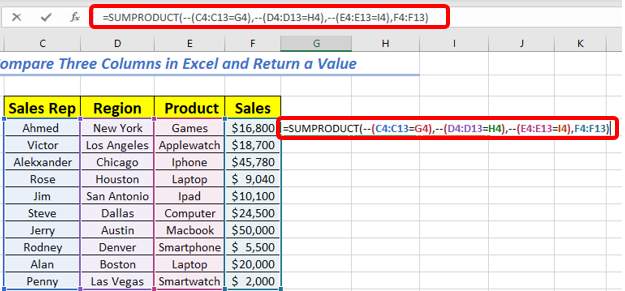
The SUMPRODUCT function is also among the lookup methods you can use to compare three excel columns. However, it only works for numeric values. It is a versatile method that extends various functionalities even further. Besides comparing more excel columns, it also multiplies ranges together and returns the sum of products, especially when counting without duplicates. To use the function to compare three columns and return a value, you can follow these steps:
1. Select a new cell where you want the resulting value to appear. For example, you can select cell J4.
2. Write the following formula in the new cell and press the Enter button:
=SUMPRODUCT(–(C4:C13=G4),–(D4:D13=H4),–(E4:E13=I4),F4:F13)

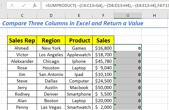
The formula will return a value in cell J4 after comparing a range of cells in three columns.
3. You can use the Fill Handle (+) icon to Autofit the formula for the rest of the cells within column J.

Combining IF and COUNTIF Functions
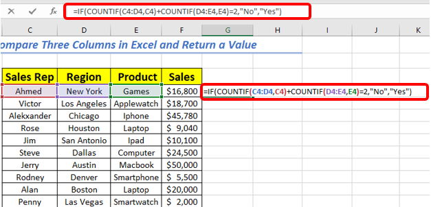
When combining IF with the COUNTIF function to compare three columns, you will need to specify the expected result with Yes for matches and No for mismatches. To identify duplicates from three columns using the combination, follow these steps:
1. Select the cell where you want the matching result to appear. When comparing columns C, D, and E, you can select cell F4.
2. Write the following formula in the cell and press the Enter button:
=IF(COUNTIF(C4:D4,C4)+COUNTIF(D4:E4,E4)=2,"No","Yes")

3. You now use the Autofill icon to drag the formula down the column and generate matching results.

Scanning Three Columns to Highlight the Matched Records
Besides setting up a new rule, you can also use the Duplicates Values option in the Conditional Formatting section to highlight the matching data when comparing three columns. Here, follow these simple steps:
1. Select the three columns you want to compare. For example, you can select columns C, D, and E.
2. Click the Conditional Formatting option on the Home ribbon.

3. When the Conditional Formatting screen opens, click on the Highlight Cells Rules option.

4. Select the Duplicate Values from the next menu list.

5. When the new Duplicate Values window opens, click the OK button. You will see all the matching records highlighted.

Combining IF $ AND Functions
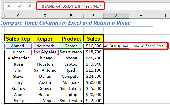
Combining IF $ AND functions allow you to identify matches using specific operations such as Match, No Match, Yes, No, False, and True. To compare three columns using this combination, follow these steps:
1. Select the cell next to the three columns you want to compare. For example, if you want to compare cells C5, D5, and E5, you can select cell F5.
2. Write the following formula in the selected cell:
=IF(AND(C5=D5,D5=E5),"Yes","No")

3. Press the Enter button. The operation will return the result in cell F5 to tell if there is a match or not.
4. You can use the Fill Handle (+) icon to autofill the formula in the rest of the cells along the column.

