
Excel has provided a vast formula to perform different operations.
1. Sum
Used for adding numbers
Syntax
Sum(Number 1, Number 2.,Number 9) or SUM( Starting location of data: Last location of data)
Example
sum(20,30,40) = 20+30+40 = 90
=SUM(A1:A8) = add all numbers updated in column A from row 1 to 8

=SUM(A1:B8) = add all numbers updated in column A and column B from row 1 to row 8.

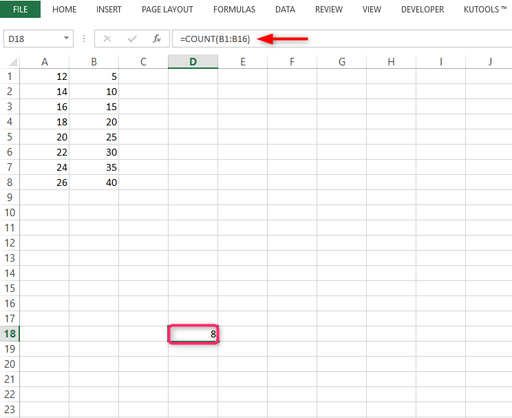
2. Count
Used to count numbers in the selected range.
Syntax
COUNT( Value 1, Value 2, …. , Value N) or COUNT(First cell of data range: Last cell of data range)
Example
COUNT(B1:B16) is equal to the count of numerical data points in column B from row 1 to row 16.
3. Average
Used to average/mean of the given set. I,e the sum of all data points divided by the count of data points.
Syntax
AVERAGE(Value 1, Value 2…., Value N) or COUNT (First cell of data range: Last cell of data range)
Example
=AVERAGE( B1:B16) = SUM( B1:B16)/COUNT(B1:B16)
This function will not consider empty cells and non-numeric cells.

4. IF Function
IF function is used to perform the required action if a predefined condition is either TRUE or FALSE.
IFERROR is used to manage error evaluated while performing another function.
Syntax
If ( Logical condition, Value_if_true, Value_if_false)
IfERROR(value, value_if_error)
For example if Function to return True or False =IF(B4>30,"True","False")

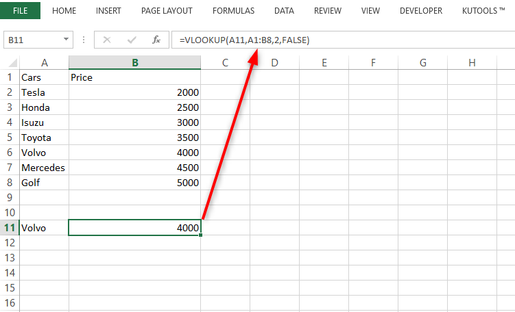
5. VLOOKUP
used to find a required value in a table in a corresponding referred now
Syntax
VLOOKUP(Lookup_value, table_array,col_index_num),[range_lookup]
Example
Let's look up the price of Volvo from the following list. Use =VLOOKUP(A11,A1:B8,2,FALSE)
6. Offset
Returns a reference to a range that is a specified number of rows and columns from a cell or range of cells.
Syntax
OFFSET(reference, rows, cols,[height],[width])
Example

7. COUNT employees
From the data, calculate the count of data equal to, not equal to, less than, or higher than a given number. COUNTIF can be used.
Example
Cells equal to 20.
=COUNTIF(B2:B16,F13)

8. MAX, MIN
MAX will return the largest numeric value of the range, MIN will return the smallest numeric value of the range. They will include only numeric values
MAXIF MINIF will return the largest and smallest values respectively only among the cells.
Syntax
MAX (Range); MIN(Range);
MAXIF([Max_Range], Criteria Range 1, Criteria Range 2, Criteria Range N)
MINIF [(MIN_Range], Criteria Range 1, Criteria Range 2, Criteria Range N)
Example
Example lets find the largest value =MAX(B2:B16)

9. Round
The ROUND function is used to round numbers to a specified number. ROUNDUP, ROUNDDOWN can be used to round numbers away from Zero.
Syntax
ROUND(Number, digit)
ROUNDUP(Number, digit)
ROUNDDOWN(Number, digit)
Example
For Example, let's round down a number to 1 decimal place =ROUNDDOWN(B4,1)

10. Replace
Used to search and replace a character to the text
Syntax
REPLACE(old_txt, Start num,num_char_to_replace, new text)
For example, let's replace the last 2 characters with an empty string. Use =REPLACE(A2,6,2,"")
