
Microsoft Excel is an excellent tool often used to keep track of data and other useful records. Among the various capabilities entailed in excel is the use of function and not only so but those that are conditional by nature. This conditional function operates under the same principle of Boolean logic. In our case, instead of 1's and O's, we have True and False. This type of formulae is very powerful in its simplicity.
For example, you might be a class teacher. You may need to calculate and see the student's performance in relation to the mean score.
Having noticed the importance of the true and false, it is time to dive into its use!!!
How to use the true and false function in Microsoft Excel
1. Have a list of data in place to compare.. as in my case, the data is below
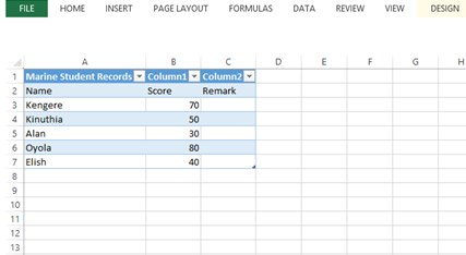
In our case, with the data provided, we will be checking those that have attained the mean mark, which is 50.
For those who have attained 50 and above, the remark would display true, and those that are 49 and below False will be what we expect.
2. In cell C3, write the conditional function If (B3>= 50, True(), False())
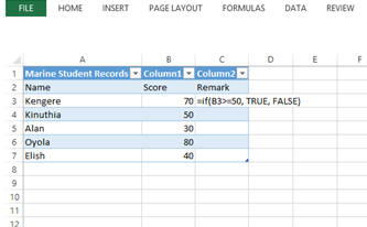
In our table, since the first column B3, Kengere is above average, the outcome will be true
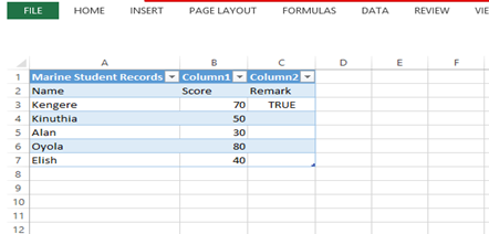
3. Repeat the same process in the remaining cells

Method 2
Excel comes with inbuilt true and false functions. For example, if you type =TRUE() a TRUE value will be returned.
Alternatively if you type =FALSE() a false value will be returned

However, you don't have to use these functions under normal circumstances. In the above table, TRUE represents 1 while False represents 0.
Knowing that we can apply it to make calculations. The formula multiplies the result of TRUE by 25 and vice versa

Using TRUE As A Boolean Function
When calculating a TRUE function, you use a numerical value of 1.
As you place the logical operator in the input, the expected outcome will either be TRUE when the logic is correct or FALSE if it’s incorrect.
For example;
Products in any given place are always accompanied by their prices. Assume that all products are sold at a discount of 15% for the price that is more than $250.
If your logical statement states prices are more than $250, then the final answer will be TRUE in the contrary TRUE will change to the percentage of 15% that was initially provided.
Let's consider an arbitrary function that returns logical outcomes either True or False;
=IF(B4>100,"True",FALSE())
Combining TRUE and NOT Functions
Both TRUE and NOT functions are used as logical functions. The NOT function expresses one value as not similar to another value. When combining the two functions, giving TRUE will return FALSE, while giving FALSE will return TRUE.
Steps;
Assuming you want to check if the value in cell C5 is not greater than $200 and give the outcome in cell E5, you can use the steps below:
1. Type the formula below in cell E5 and press the Enter button:
=IF(NOT(C5>=200),TRUE)
2. Use the Autofill Handle to drag the formula in other cells down the columns.

Conditional Formatting Using TRUE
Steps;
1. Firstly, go to the styles and locate the Conditional Formatting toolbar.
2. Now, go back to the dataset and highlight the data you need.
3. Click on the Home tab menu, and select the Conditional Formatting option.
4. Select New Rules that will open a New Formatting Rule dialog box.

5. Continue and select the Use a formula to determine the cells to format option.
6. Place the following formula for the odd number.
=ISODD(B4)

7. Finally, open the format option then Fill to choose the color to use.
Comparing Strings Using IF and False Function
Assuming you have a dataset showing products and their delivery status indicated in column C. Delivery status could be Delivered, Shipped, Processing, and Pending. If you want to check whether products are delivered, you can use the steps below:
1. Type the formula in the cell where you want to see the outcome if the delivery is complete. For example, you can use cell D4 as your first case and copy it till cell D11
=IF(C2="Delivered “,”True”,FALSE())

Where;
C4=”Delivered” is the condition.
“True” will appear when the condition is correct or true.
FALSE() this function will give back false if the condition is false

Using COUNTIF and FALSE Functions
In the above formula, you used “Delivered” as the condition. But in this method, you will count the unfinished deliveries. However, you will need to count the cells where Delivery Completed is equal to FALSE.
1. Write the following formula in the cell where you want to return whether the marked completed delivery is false. For example, you can use cell H6 as your first case.
=COUNTIF(D2:D9,FALSE())
Where;
D2:D9 is the range where FALSE values are.
FALSE()) is the range between the compared cell values with the FALSE function return value.
2. Copy the formula down the column to the remaining cells using the Autofill Handle.

Comparing Two Numbers Using IF and FALSE Function
Assume you have a range of data on different products from the last two years' total sales.
Steps;
1. Place the formula in cell E3 and copy it to E10.
=IF(D4>C4,"True",FALSE())
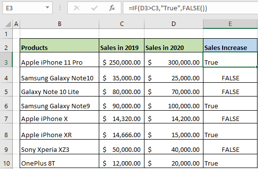
Where;
D4>C4 is your logical condition.
Since you want to determine the sales in the D column that are more than the C column, when it's yes it prints the “True” message but when FALSE it gives back FALSE.
Find False Value
1. Place the formula in cell F4 and copy it down to F12.
=NOT(E4)

Where;
E4 is logical.
If your results are either logical or numerical value is zero then the logical value is FALSE. When the numeric value is any number the logical value is TRUE.
Conclusion
That was simple, is it so? Hoping the guide has been simple and useful as you notice how powerful a tool the true and false function is, and advancing your knowledge in its application will only make Excel desirable and easy to use