Concatenate is an excel function that allows you to join two or more strings together.
When creating a Pivot table, you may want to combine data from two or more columns to form a single column. An example, you may wish to combine the names field with the address field to form a single column or combine some texts with a formula-driven value.
Before you merge values of Pivot Table, you should have an already-enabled Pivot Table, or else you should create one. Follow the steps below to create a Pivot Table.
Open your Excel workbook.

Pivot Tables have certain criteria. Thus, opened Excel workbooks should include the below data components.
- Your data should be put in an Excel table.
- The table should have a continuous data range with column headers or titles.
- It should have a database structure for your data. That means each header column should have a criterion or a value.
- The Excel table should consist of a list of values.
Now click any cell inside your data workbook.
At the top menu of your workbook, go to the Insert Tab

Under the Insert Tab ribbon, select Tables at the far top-left corner and choose Pivot Table. A dialog box will appear, and Excel will automatically select the data for you.

Next, a Create Pivot Table menu appears. The default location for a new Pivot Table is a new worksheet. You should then click on the New Worksheet check box and click OK at the bottom right. The Pivot Table field pane will appear after the action.

You should now export your data. Under the Pivot Table field, choose your title fields to add to the report and drag the fields to your desired areas below.
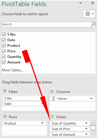
Now that you have your Pivot Table, you can concatenate its values using these methods:
Simple Concatenate
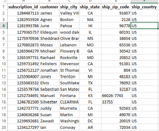
In this table, you can create a PivotTable with combined Ship_city and Ship_state text values. To do that, you need to use CONCATENATE function, which will allow you to join the columns together.
Syntax
=CONCATENATE (Text1, [text2, … text_n])

NOTE: If you're using Excel 2016, use the CONCAT function.
The address column will be used to create the PivotTable, a Pivot chart, or a Pivot View report, just like you would add any other column.
Concatenate with Space characters
To add spacing between the join text type, this command
=CONCATENATE (C2, " ", D2) on cell G2.
You can also add a comma to make the joined text more readable
=CONCATENATE (C2, ", ", D2)
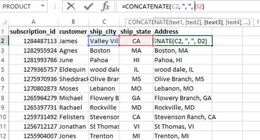
Add a PivotTable with the combined address column
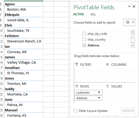
Format the PivotTable to display the data in columns.
Go to Pivot tools and click the design menu. On the layout group, choose report layout and select show in tabular form. The data will be displayed as shown below.
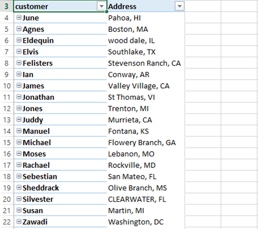
Concatenate strings with a line break
In windows, use CHAR (10) where 10 is the ASCII code for line feed.
Mac computers use CHAR (13) where 13 is the ASCII code for carriage return
In the above example, to get the combined mailing address of a customer, use the following formula;
=B2& " " & CHAR (10) &C2 & "," &D2

You must ensure the Wrap Text option is enabled for the text to display correctly with line breaks. Click on the cell, then go to cells group in the Home menu. Choose format cells. On the opened window, click alignment table then select Wrap text check box and click ok.
Once you concatenate the text, you can go ahead to create a PivotTable with the details in the joined column.
Calculated Columns in a Pivot Table
A Calculated column is often used when you want to add calculated results in an area in your PivotTable. This can be an added row or column in your PivotTable.
In the table below, we want to add a calculated column to display the total of sold Items.
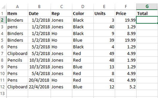
Click insert Pivot table; on the open window, select the fields you want for your Pivot table.
Once you select the desired fields, go to Analyze Menu. Under calculations, choose fields, Items & Sets tab, then click on calculated fields.
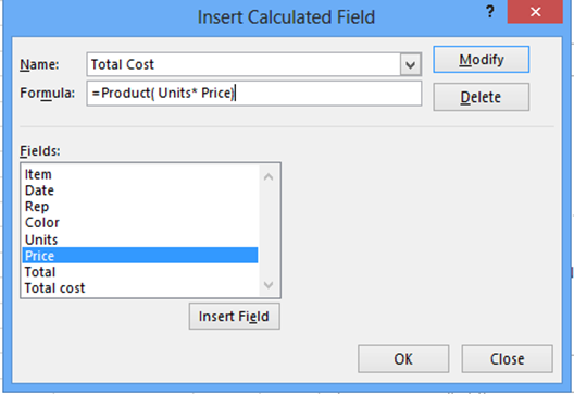
Enter the values and click ok.
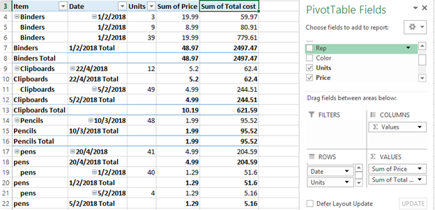
Your PivotTable will display the total of combined units and price.
Using The Ampersand Sign (&)
The ampersand sign (&) is the easiest technique you can use to combine values from two columns into one. It is represented by the formula:
=C1&” “&C2, where;
C1 is the cell reference of the first column or row, and C2 is the cell reference of the second column. Since you are concatenating values of two columns but on the same row, you can alter the formula based on your dataset. For example, you can use the formula:
=B4&" "&C4, where;
B4 and C4 represent the values in the first and second columns on the same row. On the other hand, using the two ampersand signs and double quotation marks means you want to leave a space between the two elements. If you want the elements to become one, you can avoid the double quotes and use only one ampersand sign. To use the formula to combine values in a Pivot Table, follow these steps:
Write the formula in the cell next to the columns you want to concatenate. For example, if you want to combine data in cells B4 and C4, you can write the formula in cell D4.

Press the Enter button, and the formula will return the value in cell D4.
You can use the Fill Handle (+) icon to drag the formula down the column to generate a result for the rest of the cells.

Using TEXTJOIN Function
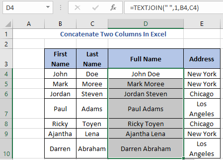
The TEXTJOIN function allows you to concatenate several values of a Pivot Table with or without a delimiter. To use the function, follow these steps:
Write the TEXTJOIN formula in the cell next to two columns you want to combine their values. For example, if you want to concatenate values in cells B4 and C4, you can write this formula in cell D4:
=TEXTJOIN(" ",1,B4,C4),

where;
The two quotation marks leave a space for the delimiter value. However, since you want to ignore the empty cell, you place 1 as the second parameter.
The formula combines values in two cells and gives the joined data in cell D4.
You can type the formula in the rest of the cells down the column or use the Autofill (+) feature to drag the formula.
Using The Flash Fill Feature
The Flash Fill is also another vital Excel feature that allows you to perform various operations, including concatenating values from two columns. When using this technique, you must manually type the values from the two columns in the next cell and press the Enter button to save the changes. Next, to combine the value from the rest of the cells, you can now follow these steps:
Click on the cell you want the combined value to appear.
Go to the Data tab and select the Flash Fill option from the Data Tools menu. You will easily generate the concatenated values for the rest of the column.

