A pivot table in its simplest form of a programming tool that permits its user to summarize selected columns and rows of data in a spreadsheet. Simply put is used in sorting information and used to breaking larger tables down into easier-to-use forms.
In answer to the popularly asked question on whether a pivot table changes the database or spreadsheet itself, the answer is in the negative. A pivot table doesn't actually change the spreadsheet or database by itself.
Create a pivot table from multiple worksheets
In a case where the data you want to summarize in this Pivot Table is in say 3 worksheets in the same workbook,

A simple method will be to make use of the Pivot Table and PivotChart Wizard.
To activate this, click on Options in the File Tab, Options, and click on Customize Ribbon

select All Commands in the “Choose commands from:” field,

Scroll till you find PivotTable and PivotChart Wizard and click “Add >>”.

Alternatively, Creating Table.
1.) Convert the data contained in the 3 worksheets into Excel Tables. To do this, starting with Sheet1, select anywhere in the data and press Ctrl + T. Confirm that the “My Table has headers” box is checked, and click OK.

2.) Do the same for the remaining 2 sheets containing the data you want to consolidate
3.) It is best to create a new worksheet where this Pivot Table will be located.

4.) Select a blank cell in the newly created worksheet
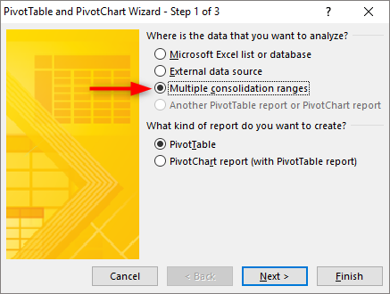
5.) Press Alt + D, and then press P. The PivotTable and PivotChart Wizard come up as shown below.

6.) Select Multiple Consolidation Ranges and Select Pivot Table then click Next

7.) Select “I will create the page fields” then Click Next

8.) Select the ranges of data you want to consolidate one after the other and click add. In this example, we have converted the data into tables, so it is much easier to reference just by typing the names of the tables: Table1, Table2, and Table3.
9.) In the “How many page fields do you want?” field, select 1. Select Table 1 in the “All Ranges” field and label it Store 1 in the Field One field as shown in the picture below. Repeat this step for the other Tables. Click Next.

10.) Select your desired position on the Pivot Table
11.) Click Finish
Now you have your Pivot Table. You can explore the Pivot Table Option and Pivot Table Field List to customize the Pivot Table to align with your requirement. In this example, we want to see Monthly values, so we are taking out the Column Field and we are left with Row, Value, and Page 1 fields.

To format the Values field, click on the Sum of Values tab under the Values field in the Field List of the Pivot Table, click on Value Field Settings, click on Number Format, and choose the Number format you want.
