
Links are beneficial to an Excel document. Links allow one to add External data to the active worksheet. However, you may want to remove or break the unwanted links from your document. Excel has various methods and tools that can be used to delete and break links. Below are some of the common ways of deleting links in Excel.
Using the Connection Tool
Below are steps to follow while using this method:
1. Open the Excel application.
2. Go to the Data tab on the Ribbon, and locate the Connections section.
3. Click the Refresh All button. Then, click the Connections button.

4. In the Workbook Connections dialogue box, you will see all the links in your document.
5. Click on the link you want to delete. If you want to delete all the links in your workbook, press the CTRL + A keys to select all the links in the box.
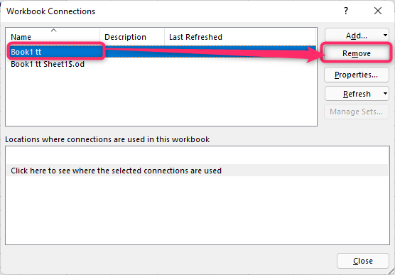
6. Click the Remove button to delete the link(s). Finally, click the Close button to close the dialogue box.
To remove Links from the Name Manager
Below are steps to follow while using this method:
1. Open the Excel application.
2. Go to the Formulas tab on the Ribbon, and locate the Defined Names section.
3. Click the Name Manager button to open the Name Manager Dialogue box.

4. Click on the link you want to delete. If you want to delete all the links in your workbook, press the CTRL + A keys to select all the links in the box.
5. Click the Delete button to delete the link(s). Finally, click the Close button to close the dialogue box.

To Remove hyperlinks
Below are steps to follow while using this method:
1. Open the Excel application.
2. Open the Worksheet that contains the hyperlink(s) you wish to delete.
3. Right-click on the cell you want to remove the link.
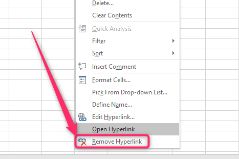
4. From the menu, choose the Remove Hyperlink option. That is all you need to do.
How to Easily Find all hyperlinks in Excel
Steps:
1. Open the Excel application.
2. Open the worksheet that contains the hyperlinks.
3. Click on the Home tab on the Ribbon, and locate the Editing section.
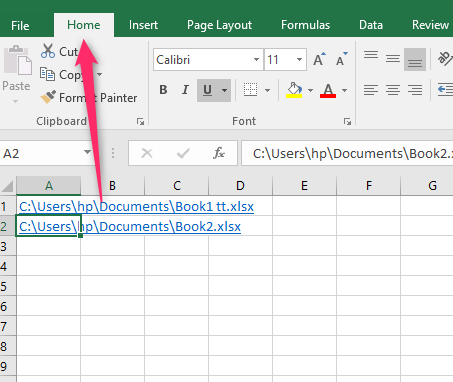
4. In the Editing section, click the Find & Select drop-down button and select the Replace option.

5. Click on the Replace tab in the Find and Replace dialogue box. Then, click the Options button in the dialogue box.

6. In the Find What options, click on the drop-down button in the Format Button. From the menu, choose the Choose Format From Cell option.

7. Then, select any of the cells with the hyperlink in your worksheet. The Format will populate in the Preview button.

8. Click the Find All button, and all the cells with the hyperlink will be shown.
