Most users know the VLOOKUP function is not that case-sensitive. For example, when you look up for DAN, dan, Dan to VLOOKUP, all this is the same. The function will return the first matching value regardless of its case.
VLOOKUP Case sensitive functions.
You can have a table like this; as you can see, we have three names with different letter cases. The VLOOKUP function won't be able to separate the three names in terms of the cases they have.
So we are going to see how we can look up case sensitive in 2 ways.
- Using a helping column.
- Use of formula.
Use of a helper column.
Helper used to get the unique value of each cell content in the lookup array. This helps to differentiate between names that have different letter cases.
Steps to follow when doing this.
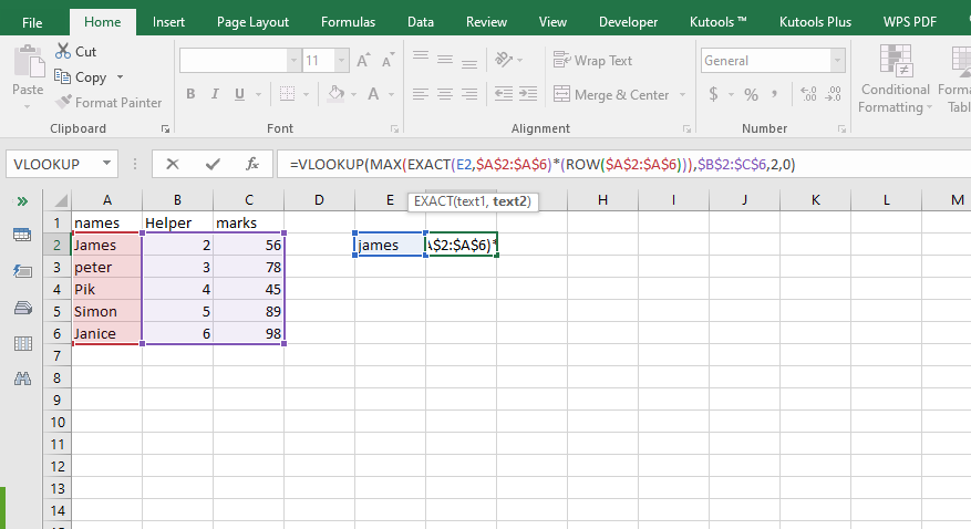
1. To your left, insert a helper column from where you would like to fetch data. As for me, I have inserted between the two columns we had.

2. Within the new column, you inserted write the formula =ROW(). This will insert the row number of each cell within the column.

3. Enter the following formula on cell F2to do case-sensitive lookup. =VLOOKUP(MAX(EXACT(E2,$A$2:$A$9)*(ROW($A$2:$A$9))),$B$2:$C$9,2,0)

4. Press Ctrl+shift+enter Enter key to apply the formula
5. Repeat the same on cells F3 and F4 but replace E2 with E3 and E4 respectively on the formula
The formula works in this way:
1. EXACT(E2,$A$2$A$9) the exact part is used to compare the lookup values E2. With other values in A2:A9.The output will either be TRUE or FALSE, where TRUE is where we have an exact match, and FALSE where we do not have the match.

2. (EXACT(E2,$A$2:$A$9)*(ROW($A$2:$A$9) The part multiplies the array of the TRUE and FALSE with other rows that is A2 TO A9. Where it is true, you will get 0.

3. (MAX(EXACT(E2,$A$2:$A$9)*(ROW($A$2:$A$9) used to return max value from the array. In our case, we will have two the exact number of rows where we have the exact match. We simply use the number as the lookup value to lookup array B2 TO C9. If you mess any value within the function, you get errors.

Use formula.
We will create a virtual helper column not far from the first procedure. The new column is not part of the workbook, but it will be created by the formula. The formula looks like this.
VLOOKUP(MAX(EXACT(D2$A$2$A$9)(ROW($A$2:$A$9))),CHOOSE({1,2},ROW($A$2:$A$9),$B$9),2,0).
By virtual means, we don't have the physical helper column, but you have created one of the columns within the formula.
Choose: will give you several cells and their content. Commas separate the cells. The semi-colon separates data in the other row. Our formula will create two columns where one column will contain a number of cells while the other will contain the results in the next column. When you use VLOOKUP is to get the lookup value of the lookup value is the output of the combination of two functions that's MAX and EXACT function. There are other formulas you can use, like match and index functions. You can check it out too.
