Each time we use excel sheets to do a recording of our collected data, there is some crucial information that we intend to keep visible all through the excel sheets. The information may be recorded in more than one row or a column.
To keep this information visible even when we scroll to the bottom is what we refer to as locking rows or freezing. Once the row is in the freeze, it will remain visible even when you browse up and down the excel sheet.
Freezing in excel sheets can be done on rows, columns, and cells provided you need to freeze them to remain always visible throughout the entire excel sheet.
In case you need to refer to that information each time you open excel sheets, it is good you freeze the rows of interest to you to avoid tedious scrolling up and down. This will enable you to save time as we all know time is expensive.
To lock the rows or to freeze the rows in excel, we have some procedures to go about that. The steps are discussed below in detail.
Step 1
Open the excel sheet that you would like to freeze the rows if the data is already created. In case you are doing it for the first time, open a new or a blank excel sheet from your device and create the data.

Step 2
The next step is now to select the rows that we would like to freeze.
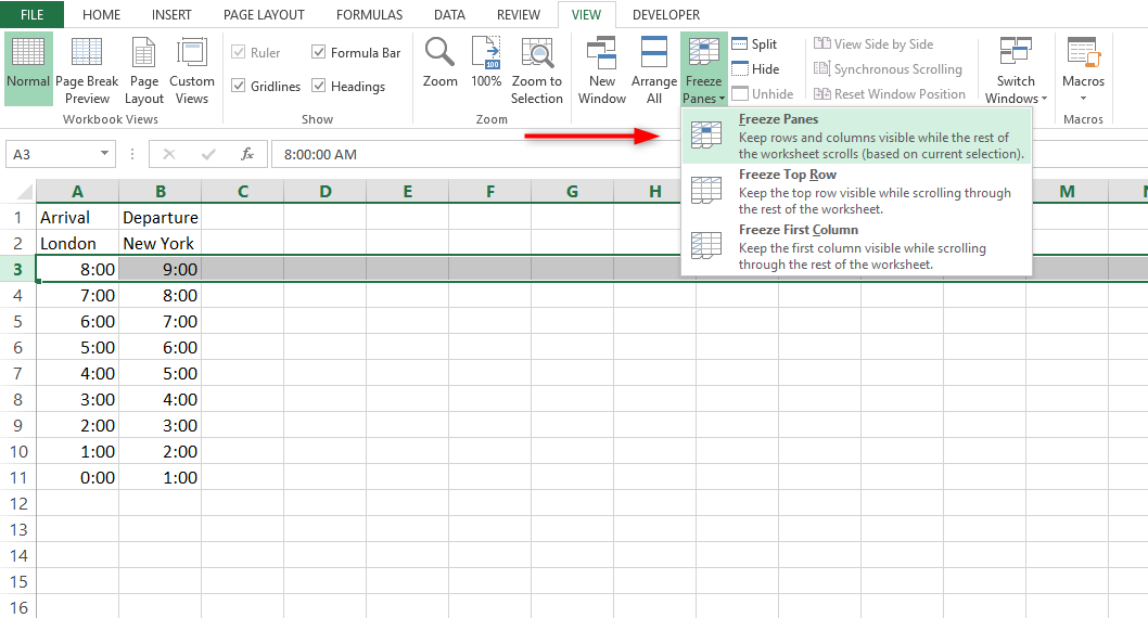
Select the third row and click on view from the menu bar.

Under view, search for freeze panes. Click on freeze panes, a list of three options will appear to select the first one which is freeze panes.

Upon clicking the freeze panes option, the top rows will be locked, this is to mean that they will remain visible even after scrolling top to bottom and vice-versa. The final data in the excel sheet will look like the one on the sample below.

