Excel tries to help users in all spheres of work on the spreadsheet, but some of the help it offers may not be wanted at the time.
For instance, if you try to paste data into a visible cell (a filtered cell), excel will also paste the data into the hidden cells (filtered-out cells). Excel thinks the action is very helpful to you! But we know that it is very hurtful. Excel does not allow users to paste values directly into visible cells only.
This action of excel has become a serious issue for many excel users. However, they can get out of this situation by using the "Paste into excel visible fields" or "paste into excel visible fields only with code."
New versions such as Excel 2013 can use the Flash fill function while the older versions can use the Fill function.
Fill Only Method
Let's take a look at the picture below. There are three columns, and we want to filter the table so that it displays odd numbers only.

1. Open the filtered table.

2. Identify and select the columns and cells you wish to work on.

3. Navigate to the home tab (ribbon) and click "fill" and "fill right." If your target is the columns by your left, then go ahead and click "fill left instead."

Viola! All the desired values will appear in the visible cells.

Meanwhile, you can click the "clear the filter" condition on your cells to be sure that nothing is copied into hidden rows.

Flash Fill Method
Users of a newer version of Excel can use the Flash fill function to quickly paste into visible cells only.
For example, you can filter odd numbers by using the steps below:
1. Identify the first cell and type '1' in the destination column.
2. Move to the next cell down and type '9'.
3. Proceed by pressing 'Enter' and then 'Ctrl + E'.
This will kick start the Flash fill function. The visible cells will be copied while the hidden rows will not be touched. You can confirm this action if you clear out the filter condition.
Use the Alt + Semicolon Keyboard Method
The Alt + Semicolon keyboard method works well when you want to copy data from outside the table.
Steps;
1. Begin by copying the values you want to paste.
2. Select the range of the cells into which you would like to paste the values, by either dragging or holding down the shift key.

3. Simultaneously press the Alt and semicolon keys, which select only the visible cells.
4. Finally, hold down the Ctrl and V to paste.

Example,
Imagine you have a table with 10 rows, you want to revise only the first three and the last two, so you hide rows four through eight.
Outside the table, you type ‘In Stock’, then you highlight the visible rows in the table and hold down the Alt and Semicolon key then press ‘Ctrl’ and ‘V’.
Use The ‘Go to Special’ Method
The Go to Special method is the on-screen variation of the ‘Alt’ + Semicolon method.
Steps;
Copy the desired values and select the cells into which you want to paste.

Select the Home tab and locate and click on the Find & Select option.
A drop-down menu will pop and select Go to Special.

Select the Visible Cells Only option and then click OK. Press Ctrl+V on the keyboard to paste the values.

Add and Use a Quick Toolbar Command
Steps;
1. To add the Select Visible Cells option, go to the Quick Access Toolbar (QAT) menu by clicking on the icon in the far upper left-hand or just below the ribbon panel (depending on the arrangement you favor) of the Excel interface.

2. In the menu, with is a downward-facing arrow with a horizontal line above it, select More Commands

3. From the dropdown Choose Command From, select All Commands, scroll down through the options and highlight the Select Visible Cells options and click Add.

4. Now the Select Visible Cells option is now easily accessible.
Apply Formula to Paste a Set of Values to the Visible Cells
We can apply a simple formula to paste a set of values in the same table. For instance, we want to copy the values in column E and paste them into column D only for one product, Cable.
Steps;
1. First, select cell D5 and type the formula
=E5

2. Press Enter and use the Autofill tool to fill the series

3. As a result, it will simply paste the values in all the cells.
Paste A Set Of Values With Excel VBA When Filter Is On
We will paste the set of values into the same table using Excel VBA Code.
Steps;
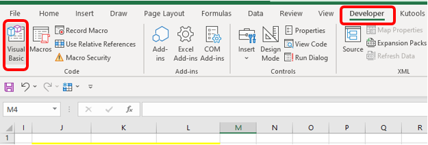
1. Under the Developer tab, select Visual Basic

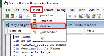
2. And then under the Insert tab, select Module

3. A new window will pop out, and then paste the code given.
Sub Paste()
Dim rg As Range
Dim visible_source As Range
Dim destination As Range
Dim source As Range
Dim r As Range
Set rg = Application.Selection
rg.SpecialCells(xlCellTypeVisible).Select
Set visible_source = Application.Selection
Set destination = Application.InputBox("Choose Destination:", Type:=8)
For Each source In visible_source
source.Copy
For Each r In destination
If r.EntireRow.RowHeight <> 0 Then
r.PasteSpecial
Set destination = r.Offset(1).Resize(destination.Rows.Count)
Exit For
End If
Next r
Next source
End Sub

Get Complete Code Source from Here

4. After that close the Visual Basic window
5. Now you can select the range you want to copy
6. Then, select Macros under the Developer tab.

A dialogue box will pop out, there select Paste in the Macro Name and press Run

7. Another dialogue box will pop out asking to choose the destination. In the Choose Destination box type: $M$5:$M$10 or select the range of cells in the table where you want to paste the values and press OK

8. At last, the required output will appear in column D
