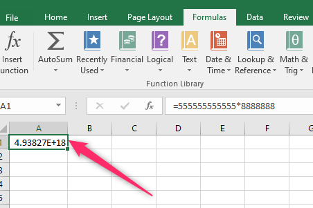
In Excel, numbers are stored in Scientific Notation. The Scientific Notation has a number limit of 15 numbers. Therefore, if your dataset exceeds 15 numbers, Excel automatically converts the number into scientific notation. When a large number is converted to scientific notation, an e (Euler’s number) is added to the number. This article will discuss ways of removing the e from your dataset.
Using the Custom Number Tool
A] Using the Home Tab
Steps to follow:
1. Open the Excel application.
2. Open the Workbook that contains the dataset with the Euler’s numbers.
3. Click or highlight the cells with the e values.

4. Click the Home tab on the Ribbon, and locate the Number section. Click the Dialogue launcher icon.

5. In the Format Cells dialogue box, click the number tab. Click the Number button. Set the number of decimals places to zero.
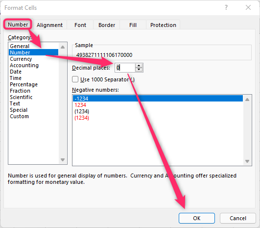
Hit the OK button.

B] Using the Right-click feature
Steps to follow:
1. Open the Excel application.
2. Open the Workbook that contains the dataset with the Euler’s numbers.
3. Click or highlight the cells with the e values.

4. Right-click and select the Format cell option.

5. In the Format Cells dialogue box, click the number tab. Click the Number button. Set the number of decimals places to zero.

Hit the OK button.
Using the TRIM Function
A] Using Formula bar
Here are the steps to follow:
1. Open the Excel application.
2. Open the Workbook that contains the dataset with the Euler’s numbers.

3. Click on an empty cell that will hold the results, and then click on the Formula bar.
4. Type the Equal sign followed by the TRIM function. That is, =TRIM (
5. Select the cell with the Euler number. For Example, =TRIM (A1)
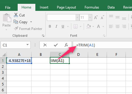
6. Finally, hit the Enter key.

B] Using the Insert Function Tool
Steps to follow:
1. Click on the Formulas tab on the screen, and then locate the Function Library section.
2. Click the Insert Function button to open the Insert Function dialogue box.

3. In the Search for a Function section, type TRIM and press the Go button.
4. Select the TRIM option in the Select a Function section and then hit the Ok button.
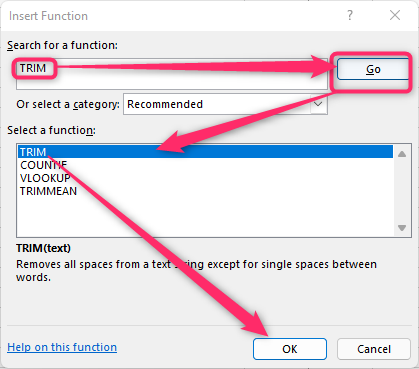
5. In the Text section, click the right button and select the cell containing the Euler’s numbers.

6. Finally, click the OK button.
Using the CONCATENATE function
Steps:
1. Open the Excel application.
2. Open the Workbook that contains the dataset with the Euler’s numbers.
3. Click on an empty cell that will hold the results, and then click on the Formula bar.
4. Type the Equal sign followed by the CONCATENATE function. That is, =CONCATENATE (
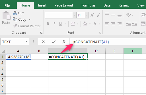
4. Select the cell with the Euler number. For Example, =CONCATENATE (A1)

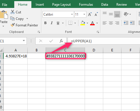
Using the UPPER Function
Steps:
1. Open the Excel application.
2. Open the Workbook that contains the dataset with the Euler’s numbers.

3. Click on an empty cell that will hold the results, and then click on the Formula bar.
4. Type the Equal sign followed by the UPPER function. That is, =UPPER (
5. Select the cell with the Euler number. For Example, =UPPER (A1)