When we are dealing with excel sheets, we may feed in data with errors or we may happen to make slight errors and which can ruin the validity of our work. At some point, you may think of erasing the whole data but that will cost you a lot when it comes to time.
Excel has had this functionality to correct the mistakes especially when we happen to exceed the length of the values we intended to write. You can remove the first characters, or the last characters to suit your data length using the built-in excel formulas.
Using the built-in formulas other than manual erasing save you time and assure your work of accuracy. Secondly, the use of built-in formulas helps the user do more automatic work or machine work than the use of manual erasing.
The following are some of the steps we can follow to do a quick shortening of values in excel sheets.
Step 1
Open a new excel sheet to record some values on one column moving downwards. It can be any type of data. For example, we will use the data below for illustration purposes.

Step 2
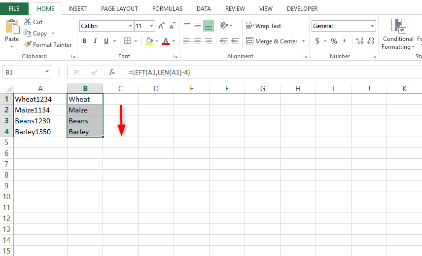
The second step will be to choose the cell, row, column to shorten. We are going to shorten the cell or row by the four last characters. With the help of this formula, =LEFT(A1,LEN (A1)-4) we can easily manage to shorten the already written values in the cells by removing the last four characters. To explain this formula, =LEFT (A2, LEN (A2) -4) we use the function LEFT to shorten the values, A1 is the cell we wish to shorten and -4 is the number of values we would like to remove. Appropriate use of the formula will give you a result like the one below.

Hold and drag the first cell to automatically remove the last four characters from the remaining cells

That is how the cells would look like with the removed characters, the process and the formula has proven to be error-free unlike the use of manual erasing of characters or the numeric digits.
