Excel is a vital tool when it comes to calculations ranging from the simplest to more complex ones. The square root is quite common when working on calculations and in excel it is easy with a few steps. The square root is a mathematical symbol that simply means a number that you multiply by itself to get the original number. There are a number of ways of applying square root in excel which include:
Use of symbols
Simply find the symbol dialog by:
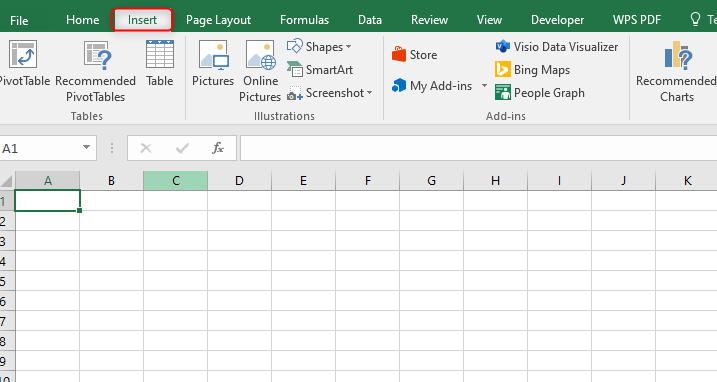
1. Go to insert then symbols

2. Click the symbol

3. After choosing symbol dialog, select mathematical operators

4. Scroll down to find the square root function
5. Choose the square root then click the insert button

Alternatively, use the character code by;
1. Select Unicode (hex) from the dropdown.
2. Type 221A into the character code box ('A' to be capital)

Using symbol font
Square root symbol is available in a front group called a symbol. To apply it just simply change a cell font to a symbol then enter "O"( "O" must be in the capital)
Note that this method is limited to keyboards that have the character "O"
Using a formula.
Normally the UNICHAR function of excel returns a Unicode character based on the numeric value given. To apply square root simply key the number 8730 into the function in the format;
=UNICHAR(8730)

Using Alt function
This trick doesn't require additional steps. Simply hold down the Alt button then type the corresponding code for the character. That is; press ALT+251and a square root will be added
Using custom formatting method
1. Select all the cells

2. Click the custom formatting option
3. Add formatting into the formatting input bar
4. Click OK
Using power function
This is an alternative method of calculating the square root. Apply the formula;
POWER (number, power)
Where; the number is the reference of the cell that contains the number you want to find the square root and power is the exponent to raise power to. An example is
POWER (A1,1/2)

Using power query
This is a dynamic method to use and note that each time you enter a new value in the table it will give the square root of that number
Use the following steps:
1. Select any cell from the table then go to Data Tab

2. Go to Get transform data and click on Table/Range.

2. After selecting it, Excel will open the power query editor then add the table into it.
3. Create a new column with square root values by;
Go to add column tab then click on the custom column

4. On the custom column window opened add:
Enter the column name square root in the column name input box. Then enter the formula =Number.Sqrt([Numbers]) in the custom column formula input box.

A new column with square roots of the numbers in the first column will be displayed
5. Delete the first column of original values by right-clicking on the column then click remove

6. Go to the home tab then click close and load

7. Get windows to load data by;
Selecting the existing worksheet then add range B1@
Tick on Add to the Data model
After applying the following steps when you enter a new value in the original data table it calculates its square root automatically in the new table after refreshing it.
