Welcome to our comprehensive guide on Excel tips and tricks. In this article, we will delve into the world of conditional formatting in Excel, exploring various ways to make your spreadsheets more dynamic, impactful, and visually appealing.
Conditional formatting is a powerful feature that allows you to apply formatting rules based on specific conditions, such as color scales, data bars, and icon sets. By leveraging these rules, you can highlight key data, identify trends, and streamline your data analysis process.
Whether you're new to Excel or an experienced user, these tips will help you enhance your spreadsheet skills and make the most of your data. So, let's get started!
Key Takeaways:
- Conditional formatting allows you to apply formatting rules based on specific conditions.
- By leveraging conditional formatting, you can highlight key data, identify trends, and streamline your data analysis process.
- Excel offers a wide range of conditional formatting options, including color scales, data bars, and icon sets.
- Customizing conditional formatting rules and managing them effectively is crucial for ensuring your spreadsheet looks exactly how you want it to.
- Advanced conditional formatting techniques, such as dynamic formatting and formatting across multiple sheets, can take your skills to the next level.
Understanding Conditional Formatting in Excel
Conditional formatting is a powerful feature in Excel that allows you to apply formatting rules based on specific conditions. These conditions can be based on values, formulas, or even other cells. By using conditional formatting, you can visually analyze your data and make your spreadsheets more dynamic and impactful.
Some of the formatting options available with conditional formatting in Excel include color scales, data bars, and icon sets. These options can help you to quickly identify trends, outliers, and other important data points at a glance.
To access the conditional formatting feature in Excel, simply select the cells you want to format and then click on the "Conditional Formatting" button in the "Home" tab. From there, you can choose from the various formatting options available and customize the rules to meet your specific needs.
Overall, understanding conditional formatting is key to making the most of this powerful feature in Excel. By knowing how to use it effectively, you can take your spreadsheet skills to the next level and become more efficient and productive in your work.
Highlighting Key Data with Conditional Formatting
Conditional formatting in Excel is a powerful tool that allows you to visually emphasize important data in your spreadsheets. In this section, we will cover some useful and practical tips on highlighting key data with conditional formatting and make your spreadsheets more dynamic and impactful.
Emphasize specific values
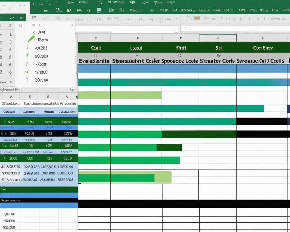
One way to highlight key data is to use conditional formatting to emphasize specific values. For example, you can use the "Highlight Cells Rules" option to highlight values greater than or less than a certain number. Alternatively, you can use the "Data Bars" option to visualize the magnitude of a value with different bar lengths, as shown in the table below.
| Region | Revenue |
|---|---|
| North | 10,000 |
| South | 15,000 |
| East | 7,500 |
| West | 12,500 |
Identify duplicates
Another way to highlight important data is to identify duplicates. This can be accomplished using the "Duplicate Values" option in the conditional formatting menu. This feature will highlight any cells in your data range that contain duplicate values, allowing you to easily identify and remove duplicates to keep your data clean and accurate.
Highlight cells based on specific criteria
You can also use conditional formatting to highlight cells based on specific criteria. For example, you can use the "Custom Formula" option to apply formatting rules based on complex conditions, such as highlight all cells that contain the word "urgent". This can be particularly useful in large datasets where you need to quickly identify and highlight specific records.
By utilizing these conditional formatting techniques, you can quickly and efficiently highlight important data in your spreadsheets, making them more impactful and informative. Experiment with these Excel tips and tricks to see which ones work best for your data analysis needs.
Customizing Conditional Formatting Rules
Conditional formatting is a powerful feature in Excel, but did you know that you can customize these rules to suit your specific needs? By creating conditional formatting rules, you can highlight important information and make your spreadsheet more visually engaging.
There are various ways to customize the formatting rules in Excel:
- Formula-Based Rules: By creating formula-based rules, you can apply conditional formatting to specific cells based on your desired criteria. For example, you can create a rule that highlights cells that contain values greater than a certain number.
- Data Validation: Using data validation, you can create rules that restrict the type of data that can be entered into a cell. You can also use data validation to highlight cells that meet certain conditions.
By customizing these formatting rules, you can ensure that your data is presented in a way that is easy to understand and visually appealing. Take time to experiment with different customization options to find the ones that work best for you.
Keep in mind that too much formatting can be overwhelming and detract from the readability of your spreadsheet. Use formatting sparingly, ensuring that it enhances your data analysis and doesn't distract from it.
Managing Conditional Formatting with Cell Rules
One of the most powerful features of Excel's conditional formatting is the ability to manage it using cell rules. With cell rules, you can modify, clear, and prioritize formatting rules to ensure that your spreadsheet looks exactly how you want it to, while maintaining the flexibility to make changes as needed.
To modify an existing rule, simply select the cell or range of cells containing the formatting rule you wish to change and then click on "Conditional Formatting" in the "Home" tab of the ribbon. From there, select "Manage Rules" and select the rule you want to modify. Once you have made your changes, click "OK" to apply them.
If you want to clear a formatting rule altogether, select the cell or range of cells containing the rule you want to delete, then click on "Conditional Formatting" and then "Clear Rules." You can choose to clear all rules or just the specific rule you want to remove.
Finally, you can also prioritize formatting rules to ensure that they are applied in the correct order. To do this, select the cell or range of cells containing the rules you want to prioritize, then click on "Conditional Formatting" and select "Manage Rules." From there, you can use the "Up" and "Down" arrows to adjust the order in which the rules are applied.
By managing your conditional formatting with cell rules, you can ensure that your spreadsheet is both visually appealing and informative, while maintaining the flexibility to make changes as needed.
Conditional Formatting Tips for Efficient Data Analysis
Conditional formatting is a powerful tool that can transform data analysis by highlighting patterns, trends, and outliers in seconds. By using some simple tips and tricks, you can make the most of this Excel feature and save valuable time on data analysis. Here are some Excel tips for efficient data analysis using conditional formatting:
Tip #1: Color Scales and Data Bars
One of the easiest ways to quickly spot patterns is to use color scales and data bars. You can use the color scale feature to highlight the lowest and highest values in a range, or select from a variety of gradient color scales to represent ranges of values. Data bars are another way to visualize data in a range using bars of different lengths to represent different values.
Tip #2: Icon Sets
Icon sets are a great way to add some visual cues to your data patterns. You can select from a variety of icons, such as arrows, traffic lights, and shapes, to highlight specific values or trends in your data set. For example, you could use green up arrows to indicate positive growth and red down arrows to indicate negative growth.
Tip #3: Custom Formatting Rules
If you have specific data analysis requirements, you can create custom formatting rules based on your needs. You can use formulas to define the conditions for which the formatting should apply, or use data validation rules to limit data input to certain values. This allows you to create unique formatting rules that suit your specific data analysis requirements.
To create custom formatting rules, follow these simple steps:
- Select the cells you want to format.
- Go to the Home tab and click on Conditional Formatting.
- Select New Rule.
- Choose the formatting rule type you want to use, such as "Use a formula to determine which cells to format".
- Enter the formula or condition you want to use for the rule.
- Select the formatting options you want to apply.
- Click OK to apply the rule to your data set.
Using these conditional formatting tips for data analysis will help you quickly identify patterns and outliers, saving valuable time and effort in analyzing your data. So, start applying these tips in your spreadsheets and take your data analysis skills to the next level!
Advanced Techniques for Conditional Formatting
Conditional formatting in Excel is a powerful tool that can help you to create compelling and informative spreadsheets. With advanced techniques, you can take this tool to the next level and make your data even more interactive. In this section, we will explore some of the most advanced conditional formatting techniques, which will help you to create dynamic and interactive spreadsheets.
Create Dynamic Conditional Formatting using Formulas
One of the most advanced techniques in conditional formatting is the use of formulas. With formulas, you can create dynamic formatting rules that can change based on the values in your spreadsheet. For example, you can create a formula that highlights cells with a value greater than a certain threshold. This type of dynamic formatting can help you to analyze your data more efficiently and quickly.
Apply Formatting across Multiple Sheets
Another advanced technique in conditional formatting is the ability to apply formatting to multiple sheets at once. This can be a huge time saver if you have a large workbook with multiple sheets that need the same formatting. You can also apply formatting to whole columns or rows to quickly highlight trends in your data.
Leverage Custom Formatting Options
Excel provides a wide range of custom formatting options that can be used in conditional formatting. For example, you can create a custom formatting rule that uses data bars to visually represent the value in a cell. You can also create custom icon sets to visually represent the status of a cell or range of cells. These custom formatting options can help you to create unique and impactful spreadsheets.
If you want to take your Excel skills to the next level and create dynamic and interactive spreadsheets, be sure to use these advanced conditional formatting techniques.
Conditional Formatting in PivotTables and Charts
Expanding your conditional formatting knowledge to PivotTables and charts can take the visual analysis of your data to new heights. Excel makes it easy to apply conditional formatting to these dynamic features, further enhancing their visual impact.
Conditional Formatting in PivotTables
PivotTables are a powerful tool for summarizing and analyzing large amounts of data. By using conditional formatting in PivotTables, you can quickly identify trends and outliers without manually sorting through rows and columns of data.
Here are some ways to improve your PivotTable analysis with conditional formatting:
- Highlight the highest or lowest values in a PivotTable field using color scales or data bars.
- Apply icon sets to compare data values in a PivotTable field.
- Use formula-based rules to highlight values that meet specific criteria, such as top 10 or above average.
By using conditional formatting in PivotTables, you can quickly identify trends and outliers, making your analysis more efficient and accurate.
Conditional Formatting in Charts
Charts in Excel are a great way to visually represent your data. By using conditional formatting in charts, you can make your data even more impactful and easier to understand.
Here are some ways to use conditional formatting in charts:
- Highlight specific data points or series using color or shape formatting.
- Use data bars to highlight certain data ranges in charts.
- Create creative chart title and axis label with formatting and icons.
With these conditional formatting techniques, you can make your charts stand out and effectively communicate your data insights at a glance.
Conclusion
Mastering conditional formatting in Excel can be a game-changer for anyone dealing with data. Its powerful features allow you to visually interpret information, uncover hidden insights and trends, and make informed decisions with confidence.
In this guide, we have covered various tips and techniques to help you get started with conditional formatting. From understanding the basics of conditional formatting to applying advanced techniques to PivotTables and charts, you now have a solid foundation to create dynamic and impactful spreadsheets.
We hope this guide has been informative and helpful. With continuous practice, you can further refine your skills and take your data analysis to the next level. So go ahead, give it a try, and let your data speak to you!
FAQ
What is conditional formatting in Excel?
Conditional formatting in Excel refers to the feature that allows users to apply formatting rules to cells based on specific conditions. It enables visual analysis of data by highlighting important information and making spreadsheets more dynamic.
How can I highlight key data using conditional formatting?
To highlight important data in Excel, you can use conditional formatting. This feature allows you to emphasize specific values, identify duplicates, or highlight cells based on criteria you define, helping your data stand out and draw attention.
Can I customize conditional formatting rules in Excel?
Yes, you can customize conditional formatting rules in Excel. You can create formula-based rules, use data validation, and set specific formatting options to meet your specific needs and requirements.
How do I manage conditional formatting in Excel?
Managing conditional formatting in Excel involves modifying, clearing, and prioritizing formatting rules. This allows you to fine-tune the appearance of your spreadsheet while maintaining flexibility for future changes.
What are some tips for efficient data analysis using conditional formatting?
When it comes to data analysis, conditional formatting can be a powerful tool. By effectively visualizing trends, identifying outliers, and analyzing data patterns, you can make your analysis more efficient and accurate.
Are there any advanced techniques for conditional formatting in Excel?
Yes, there are advanced techniques for conditional formatting in Excel. These include creating dynamic formatting using formulas, applying formatting across multiple sheets, and utilizing custom formatting options to enhance the visual impact of your spreadsheets.
How can I use conditional formatting in PivotTables and charts?
Conditional formatting can also be applied to PivotTables and charts in Excel. This allows you to summarize and visualize data in these dynamic features, further enhancing their visual impact and making your data more comprehensible.
What are the benefits of mastering conditional formatting in Excel?
Mastering conditional formatting in Excel opens up a world of possibilities for data visualization and analysis. By effectively utilizing this feature, you can elevate your spreadsheet skills and unleash the full potential of Excel's conditional formatting capabilities.