
Find and replace is an excel feature used to search for specific data in an excel worksheet or within a workbook and what you do with the data found. This article will explore different ways you can use find and replace together with using advanced find features.
Scanning through columns and rows in a large excel document to look for certain data may be difficult but using the "excel find and replace" feature, you can easily find any data you need within a big excel sheet in seconds.
Using the Excel Find in a range of cells
The find tool can help you look for certain information in your worksheet. To do this, select a range of cells to look in.
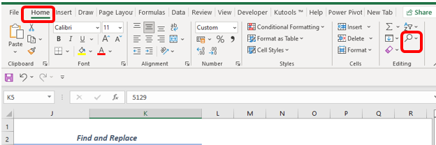
Go to the home tab > Editing group > click Find & Select > click Find. Alternatively, you can press the CTRL+F keyboard shortcut.

In the Find what box, type the characters you want to look for and click Find All or Find Next

Find All opens all the occurrences of the typed character and you can navigate to the corresponding cell by clicking any item in the list.
Find Next when you click this option, Excel selects the first occurrence of the search value on the sheet and when you click again it selects the second occurrence on the cell. This goes on until the last item is searched.
Using Find and Replace tool
The find and replace changes the value of one cell to another within a range of cells in a worksheet. The replace tab can change characters, texts, and numbers in excel cells.
Steps
1. Select the range of cells where you want to replace the text or numbers.
2. Go to Home menu > editing ground > select Find & Select > Click Replace or press CTRL+H from the keyboard

3. On Find what box type the text or value you want to search for. In the Replace with box, type the text or value you want to replace with.

4. Click Replace button to replace a single text or click Replace All to replace the entire sheet with that value or text.
How to Find and Replace Multiple Values at once with VBA Code
Find and Replace can be used to find multiple values and replace them with values you desire using Excel VBA code.
Steps
1. Create the conditions that you need to use. This should be made of a list of old values and replace values.

2. Click on the Developer tab then select Visual basic under code group or hold down the ALT+F11 function key to open the Visual Basic window.
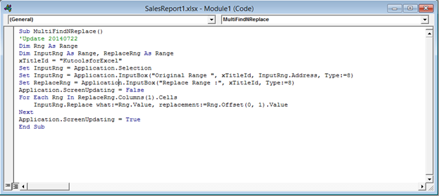
3. Click Insert > module, and paste the following code in the module window.
Sub MultiFindNReplace()
'Update 20140722
Dim Rng As Range
Dim InputRng As Range, ReplaceRng As Range
xTitleId = "KutoolsforExcel"
Set InputRng = Application.Selection
Set InputRng = Application.InputBox("Original Range ", xTitleId, InputRng.Address, Type:=8)
Set ReplaceRng = Application.InputBox("Replace Range :", xTitleId, Type:=8)
Application.ScreenUpdating = False
For Each Rng In ReplaceRng.Columns(1).Cells
InputRng.Replace what:=Rng.Value, replacement:=Rng.Offset(0, 1).Value
Next
Application.ScreenUpdating = True
End Sub
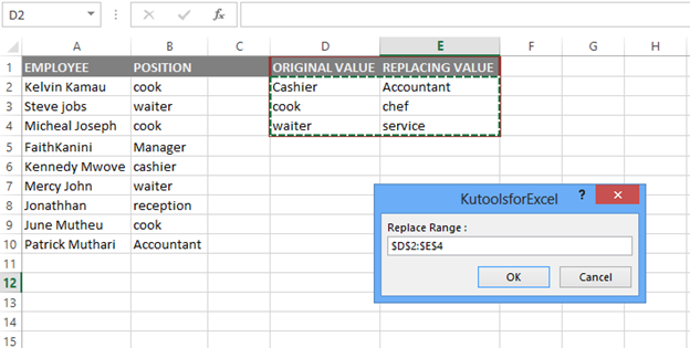
4. Click Run or press the F5 Key to run this code. Specify the data range in the pop-up window.

5. Click OK and another prompt dialog box will appear for you to select the criteria you have created in step 1.
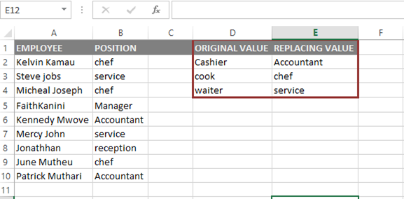
6. Then click ok. From the below screenshot, you can see all the values have been replaced with the new values.
Using Excel REPLACE Function
The REPLACE function in Excel allows you to find certain characters or a single character in a text string and change it with a different set of characters.
Syntax
REPLACE (old_text, start_num, num_chars, new_text)
Function arguments
Old_text – the original text (or a reference to a cell with the original text) in which you want to replace some characters.
Start_num – the position of the first character within old_text that you want to replace.
Num_chars – the number of characters you want to replace.
Example: We want to replace the chef position in cell B22 to be a cook

Click ok.

Apply Nested Substitute Formula to Find and Replace
The SUBSTITUTE function replaces existing text with new text in the text string. We can nest the SUBSTITUTE function for multiple values to be replaced.
Example
1. Consider the data in the tables below. Column L has some random text data. The table on the right represents the value that has to be replaced with the new ones.

2. In the first output cell, Cell M5 the related formula will be:
=SUBSTITUTE(SUBSTITUTE(SUBSTITUTE(L5:L10,O5,P5),O6,P6),O7,P7)

3. Press Enter and you’ll get an array with the new text values at once. We have used the SUBSTITUTE formula thrice as we had to replace three different values under the table on the right

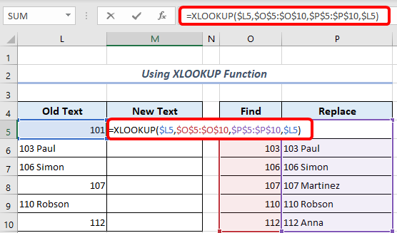
Using XLOOKUP Function to Search and Replace
The XLOOKUP function searches a range for a match and returns the corresponding item in the second range.
Example:
The old text column contains some text values. The second table on the right represents the data to be replaced simultaneously.

The required formula with XLOOKUP function in the first output cell, M5 should be:
=XLOOKUP($L10,$O$5:$O$10,$P$5:$P$10,$L10)
After pressing Enter and auto-filling the entire column will be displayed with the data the correct way.

To Find and Replace Formatting in Excel
This is an awesome feature when you want to replace existing formatting with some other formatting. For example, you may want to replace formats such as background colour, borders, font type/size/colour, and even merge cells, you can use the Find and Replace to do it.
Steps;
1. Select the cells or even an entire worksheet for which you want to replace the formatting
2. Go to Home-> Find and Select -> Replace (keyboard shortcut control + H)
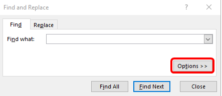
3. Click on the Options button
4. Then click on the Find What format button and a drop-down with two options will show Format and Choose format from Cell.

5. You can either specify the format manually by clicking the Format button or you can select the format from a cell in the worksheet. To select a format from the cell, select the Choose Format from Cell option and then click on the cell from which you want to pick the format.

6. Once the format is selected manually from the dialogue box or from the cell, you will see the preview on the left of the Format button.
7. Then you need to specify the format that you want other than the one selected in step 6. Click on the Replace with Format button, a drop-down with two options will show; Format and Choose from Cell

8. You can either manually specify it or pick an existing format. Once a format is selected, you will see that as the Preview on the left of the format button
9. Click the Replace All button.

Combine IFNA And VLOOKUP Functions to Find and Substitute Multiple Values
The VLOOKUP (Vertical LOOKUP) function is an alternative to the XLOOKUP function
It determines the values at the leftmost column in a dataset and returns the value in the same row from a specific column. It will return a N/A error if the lookup value is not found. Therefore, to avoid such an error, you can include the IFNA function that corrects all the errors in the VLOOKUP Function.
Steps
1. Select the cell to type the formula, such as cell C5, and combine IFNA and VLOOKUP functions as seen below;
=IFNA(VLOOKUP($B5,$E$5:$F$10,2,FALSE),B5)

2. Press the Enter button and you will see the result displayed in cell C5.
3. You can now use the Fill Handle (+) icon to drag the formula down the column.

Using the LAMBDA Function to Multiple Replace
Those using Excel 365 can benefit from an already-enabled LAMBDA function (a traditional formula language) to find and replace multiple values. The method allows them to convert a very lengthy and complex formula to a simple and compact formula. It also creates new functions that do not exist in Excel, just like the VBA code. The only downside is that it is only available in Excel 365 and you cannot use it in different worksheets.
For example, if you want to find and replace multiple words, you can create a custom LAMBDA function and name it MultiReplace. The new name can take two formulas as shown below:
=LAMBDA(text, old, new, IF(old<>"", MultiReplace(SUBSTITUTE(text, old, new), OFFSET(old, 1, 0), OFFSET(new, 1, 0)), text))
Or
=LAMBDA(text, old, new, IF(old="", text, MultiReplace(SUBSTITUTE(text, old, new), OFFSET(old, 1, 0), OFFSET(new, 1, 0))))
Although both formulas might look the same (recursive functions), you can note the difference using their exit points. For instance, the IF function in the first formula checks whether the old text is not blank (old<>””). If it is blank (TRUE), the MultiReplace function is called. If it is not blank (FALSE), the function gives a text in its current form and exits.
On the other hand, the IF function in the second formula uses reverse logic: if old is blank (old=""), then it returns a text and exits. But if the old is not blank, call MultiReplace. Therefore, to use any of the formulas, you need to name the MultiReplace function in the Name Manager first. Then, once you get the name, you can now proceed to use it to find and replace multiple values as discussed below.
1. First, know the syntax of the MultiReplace function is:
MultiReplace(text, old, new), where;
text is the source data.
old is the value you need to find.
new are the values you need to replace with.
2. Type the formula in the cell (column) next to the data you want to find and replace. For example, if you want to replace values in column A, you can type the following formula in column B, say cell B2:
=MultiReplace(A2:A10, D2, E2)
3. Hit the Enter button and a new text will appear in cell B2.
4. Proceed to drag the formula down the column using an Autofill Handle.
Mass Find and Replace with UDF
You can also use a user-defined function (UDF) to mass-find and replace multiple values in Excel using traditional VBA code. The UDF is close to the LAMBDA-defined function, but you can differentiate them by naming the UDF technique as MassReplace. It is represented by the code:
Function MassReplace(InputRng As Range, FindRng As Range, ReplaceRng As Range) As Variant()
Dim arRes() As Variant 'array to store the results
Dim arSearchReplace(), sTmp As String 'array where to store the find/replace pairs, temporary string
Dim iFindCurRow, cntFindRows As Long 'index of the current row of the SearchReplace array, count of rows
Dim iInputCurRow, iInputCurCol, cntInputRows, cntInputCols As Long 'index of the current row in the source range, index of the current column in the source range, count of rows, count of columns
cntInputRows = InputRng.Rows.Count
cntInputCols = InputRng.Columns.Count
cntFindRows = FindRng.Rows.Count
ReDim arRes(1 To cntInputRows, 1 To cntInputCols)
ReDim arSearchReplace(1 To cntFindRows, 1 To 2) 'preparing the array of find/replace pairs
For iFindCurRow = 1 To cntFindRows
arSearchReplace(iFindCurRow, 1) = FindRng.Cells(iFindCurRow, 1).Value
arSearchReplace(iFindCurRow, 2) = ReplaceRng.Cells(iFindCurRow, 1).Value
Next
'Searching and replacing in the source range
For iInputCurRow = 1 To cntInputRows
For iInputCurCol = 1 To cntInputCols
sTmp = InputRng.Cells(iInputCurRow, iInputCurCol).Value
'Replacing all find/replace pairs in each cell
For iFindCurRow = 1 To cntFindRows
sTmp = Replace(sTmp, arSearchReplace(iFindCurRow, 1), arSearchReplace(iFindCurRow, 2))
Next
arRes(iInputCurRow, iInputCurCol) = sTmp
Next
Next
MassReplace = arRes
End Function
The UDF or MassReplace function works in the workbooks you have inserted the code only. Hence, to apply it, you can use similar steps used to run a VBA code. Once you insert the code, the following formula will appear in the formula intellisense:
MassReplace(input_ range,find_range,replace_range), where;
Input_range is the source range you want to replace values.
Find_range is the entire string that includes the subject and words to check and look for.
Replace_range are new characters, strings, or texts to replace with.
Steps:
1. When using Excel 365 or versions that support dynamic arrays, you can enter the following formula in the cell next to the data you want to find and replace. For example, you can select cell B2 and write this formula:
=MassReplace(A2:A10,D2:D4,E2:E4)
2. Press the Enter button to display a new text or characters in cell B2.
3. You can now use the Autofill Handle to drag the formula down the column.
4. When using old Excel versions that do not support dynamic arrays, you can manually select the entire cell range, say B2:B10, and press Ctrl + Shift + Enter buttons simultaneously.
Multiple Find and Replace with Substring Tool
Using the substring tool is also among the easiest methods to find and replace multiple values in Excel. However, before replacing values, you should consider if you are dealing with a Case-sensitive box or not. For instance, you should decide if you want to treat uppercase and lowercase as different characters.
Steps:
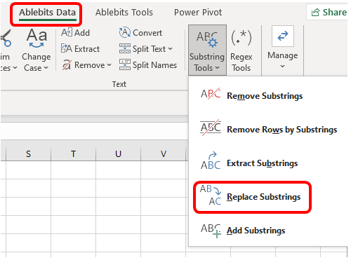
1. Go to the Ablebits Data tab, click Substrings Tools and select Replace Substrings.
2. A new Replace Substrings dialog box will emerge asking you to specify the Source range and Substrings range.
3. After filling the two checkboxes hit the Replace button and you will see your results on a new column on the right side of the initial data.
