Excel is a tool characterized by numerous cells grouped into columns and rows. Sometimes, you may be working on a large dataset that may be bigger than the size of the cell. Two ways can be used to add a new line in Excel or increase the cell size. This article will guide you on the steps and workarounds to follow while adding a new line.
To add a new line in the Excel cell
Using the Keyboard Shortcuts
Here are the steps to follow:
1. Open the Excel application.
2. Open the workbook and worksheet that you need to add a new line.
3. Place the cursor where you want to break the line and add another line.
4. Press the Alt + Enter key to add a new line in the Excel cell.
Using the Format Cells Tool
Steps:
1. Open the Excel application.
2. Open the workbook and worksheet that you need to add a new line.
3. Click on the cell that you need to add a line. Right-click on the selected cell, and choose the Format Cells button.

4. In the Format Cells dialogue box, click on the Alignment tab and locate the Text control section.

5. From the section, check the Wrap Text checkbox. Finally, hit the OK button.
To add Line in Excel Chart
Steps to follow:
1. Open the Excel application.
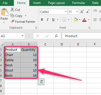
2. Open the Workbook that contains the dataset you wish to convert to a chart.
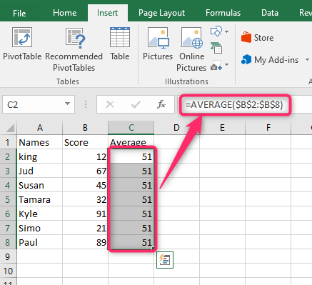
3. Locate another empty column and name it Average. Type the average function, add the arguments, and then enter. Drag the formula to other cells of the column.
4. Highlight the dataset, click the Insert tab on the Ribbon, and locate the Chart section.
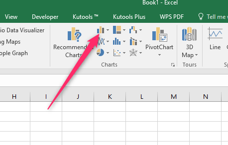
5. Click the Column chart drop-down button and select the More Column Charts option.

6. An Insert Chart dialogue box opens. In the dialogue box, click the Combo option in the left pane.
7. Click on the average section in the choose type section and select the Line option.
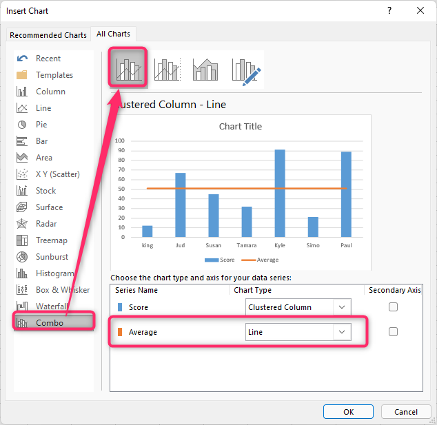
8. Finally, click the OK button. That's all you'll have a line in your chart.

To add Trendline to a chart
Here are the steps to follow:
1. Open the Excel application.
2. To get started, you need to create a chart. Therefore, add the dataset of your chart to the empty cells.
3. Highlight the dataset you've entered. Click the Insert tab on the Ribbon, and locate the Charts section. Under this section, choose any of the 2-D charts.

4. The chart will automatically be inserted into the worksheet. Then, click anywhere on the inserted chart.
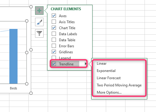
5. Locate the Plus sign symbol (Chart Element tool) on the left side of the chart.

6. In the Chart Element menu, check the Trendline checkbox. The Trendline will be added to your chart.

7. Then, hover the cursor over the Trendline button and select the type of Trendline you want to apply to your chart.