
The conditional Formatting Tool is used to perform various functions in Excel. One of the most significant tasks performed by conditional formatting is highlighting cells with the matching rule. However, did you know you use conditional formatting with multiple sheets? Excel allows one to use one rule to format other sheets within the workbook. This article will discuss the ways of applying conditional formatting across multiple sheets in Excel.
Using the Copy and Paste Tool
This is the simplest way of applying conditional formatting to multiple sheets in Excel. Below are steps to follow while using this method:
1. Open the Excel application.
2. Open the Workbook containing the worksheet you wish to add the condition formatting property. Open Sheet 1 of the workbook, and select the cells you need to add the formatting rule.
3. Click the Home tab on the Ribbon, and locate the Styles section. Under this section, click the Conditional Formatting drop-down button.

4. Choose the New Rule button from the menu to open the Edit Formatting Rule dialogue box.
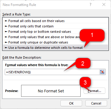
5. In the Edit Formatting Rule dialogue box, choose the “Use a Formula to determine which cells to format” option in the “Select a Rule Type” section.
6. In the Edit Rule Description section, type the formatting formula you want to use in the workbook. For example, let us use this formula = ISEVEN(ROW())
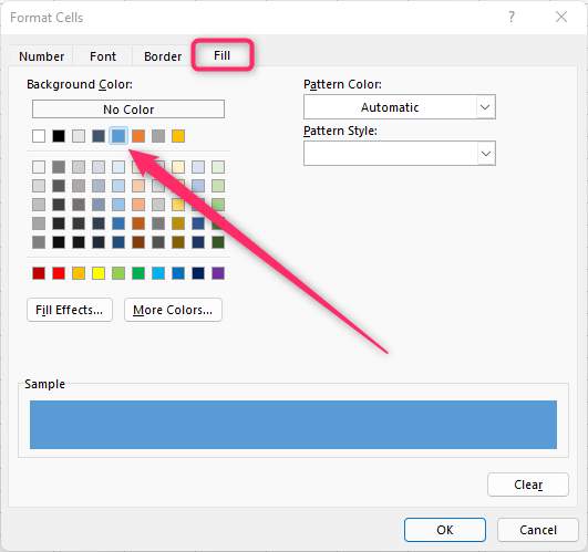
7. Click the Format button to open the Format Cells dialogue box. In the dialogue box, click the Fill tab. Next, select the color you wish to highlight the dates. Finally, click the OK button.

8. The cells in the selected sheet will be formatted. Highlight the formatted cells, and press CTRL + C keys to copy the formatting.
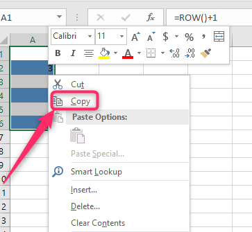
9. Open the next worksheet to which you wish to apply the formatting, and highlight all the cells with your dataset. Right-click and choose the Formatting Icon in the Paste Options section from the menu.

Using the Format Painter Tool
Steps:
1. Open the Excel application.
2. Open the Workbook containing the worksheet you wish to add the condition formatting property. Open Sheet 1 of the workbook, and select the cells you need to add the formatting rule.
3. Click the Home tab on the Ribbon, and locate the Styles section. Under this section, click the Conditional Formatting drop-down button.

4. Choose the New Rule button from the menu to open the Edit Formatting Rule dialogue box.
5. In the Edit Formatting Rule dialogue box, choose the “Use a Formula to determine which cells to format” option in the “Select a Rule Type” section.
6. In the Edit Rule Description section, type the formatting formula you want to use in the workbook. For example, let us use this formula = ISEVEN(ROW())

7. Click the Format button to open the Format Cells dialogue box. In the dialogue box, click the Fill tab. Next, select the color you wish to highlight the dates. Finally, click the OK button.
8. Select the Formatted cells, and then click the Format Painter tool in the Home tab. On clicking, a brush-like icon will appear on the active screen.
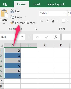
9. Open the next worksheet to which you wish to apply the formatting, and hover the brush over the cells you want to format.
