The compound Annual Growth Rate is an investment's mean annual growth rate over a given period. Excel has eased the process of computing CAGR. It is expressed in annual percentage terms. However, there is no direct function of computing CAGR in excel. But instead, several ways and workarounds can be used to compute the CAGR. Let us now discuss some of the methods in Excel that can be used to the value of CAGR.
Using the RRI function
RRI Function is one of the easiest ways of computing the value of CAGR in Excel.
Syntax:
=RRI ( Nper, Pv, Fv)
Nper: Total number of investment periods.
Pv: This is the present value of the investment.
FV: This is the Final or Future value of the investment.
Below are the steps to follow while using this method:
1. Open the Excel application.
2. Open the Workbook that contains your CAGR dataset.
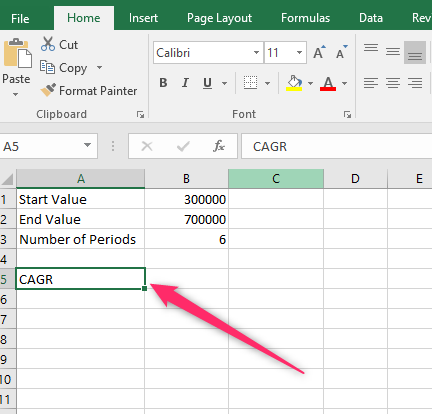
3. Locate an empty cell and name it CAGR. Then, click on the cell next to the one named CAGR.

4. On the Formula bar, type the Equal sign (=) followed by the RRI function. That is, =RRI (
5. Select the cells with your dataset and close the function. For example, =RRI (B3, B1, B2)

6. Finally, hit the Enter Button.

Using the Power Function
Syntax:
=POWER (number, power)-1
Number – ending value (EV) / beginning value (BV)
Power – 1/number of periods (n)
Below are the steps to follow while using this method:
1. Open the Excel application.
2. Open the Workbook that contains your CAGR dataset.
3. Locate an empty cell and name it CAGR. Then, click on the cell next to the one named CAGR.

4. On the Formula bar, type the Equal sign (=) followed by the POWER function. That is, =POWER(
5. Select the cells with your dataset and close the function. That is, =POWER (EV/BV, 1/n)-1
Check the example in the snap below:

6. Finally, hit the Enter Button.

Using the Rate Function
Here is the syntax of the Rate Function:
=RATE (nper, pmt, pv, [fv], [type], [guess])
Nper: Total number of investment periods.
Pmt: Amount made on each period.
Pv: This is the present value of the investment.
FV (Optional): This is the Final or Future value of the investment.
Type: This argument indicates when the amount is due.
Guess: This is your guess on what the Rate might be.
Below are the steps to follow while using this method:
1. Open the Excel application.
2. Open the Workbook that contains your CAGR dataset.
3. Locate an empty cell and name it CAGR. Then, click on the cell next to the one named CAGR.

4. On the Formula bar, type the Equal sign (=) followed by the RATE function. That is, =Rate (
5. Select the cells with your dataset and close the function. For Example, =RATE(5,,-B2,B3)
Check the example in the snap below:

6. Finally, hit the Enter Button.

