
An auto-update chart range or a dynamic chart range is a chart range that automatically updates every time the data source is changed. This type of data range is commonly used where the data source is likely to change frequently. As the chart range auto-updates, the chart also updates automatically. In this post, we will discuss some of the ways used to create auto-update chart ranges in Excel.
Using the Table Feature
The table feature in Excel is the best approach to creating an auto-update chart range. The Excel Table automatically updates the chart once new data is added to the chart source. Below are steps to follow while using this method:
1. Open the Excel application.
2. Enter the dataset you wish to convert to a chart.
3. Highlight the dataset. To highlight your dataset, left-click the mouse, move the cursor, and select the region with the dataset.

4. Click on the Insert tab on the Ribbon, and locate the Tables section. Under this section, click on the Table button. The selected dataset will automatically be converted to a table. Now, let us create a chart from the table.

5. Select the entire table, and click the Insert tab. In the Charts section, click on any chart that fits your dataset (In our case, let us use the line graph). That is all you need.

6. Now, try adding or deleting values in the dataset table.

Using the Excel Formulas
Excel formulas are built-in functions that are available in Excel and can be used to perform specific functions. Excel formulas can be used to create an auto-update chart range.
Steps:
1. Open the Excel application.
2. Enter the dataset you wish to convert to a chart. Then, click on the Formulas tab on the Ribbon.
3. Click on the Name Manager Button to open the Name Manager dialogue box in the Defined Names section.

4. In the dialogue box, click on the New button. Add the name of the Column that will contain the dynamic range in the Name section.

5. Select the worksheet containing your dataset in the scope drop-down button.
6. In the Refer to section, type this formula =OFFSET (Formula!$A$2,,,COUNTIF(Formula!$A$2:$A$100,”<>”)) and hit the OK button. This formula will set the dynamic range to Column A. Repeat this procedure to other columns in your worksheet.

7. Select the entire table, and click the Insert tab. In the Charts section, click on any chart that fits your dataset.

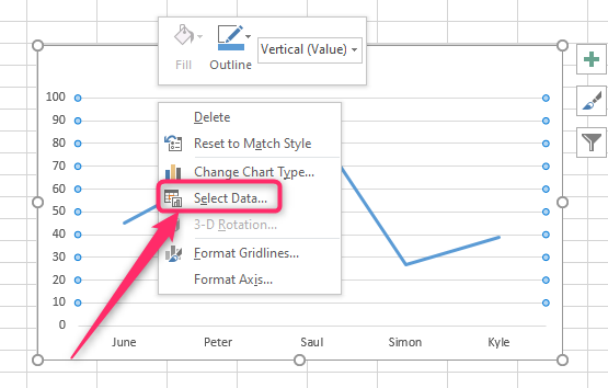
8. Right-click on the chart, and click Select Data from the menu.
9. In the Select Data Source dialogue box, click on the first column name of your dataset, and then click on the Edit button.

10. In the Edit Series dialogue box, enter the sheet’s name followed by the Column in the Series Values section. For example, =Sheet1!column1. Repeat this procedure for other columns with your dataset. For example, series values: =Sheet1!column2.

11. Click Ok to close the Edit Series box. In the Select Data Source dialogue box, click on the Edit button in the Horizontal Axis Labels section. Set the rows in the Edit Series box. For example, =Sheet1!row1. Repeat this procedure for other rows with your dataset.

12 That is all you need to do.