Advanced excel formulas can be used to lookup values or text in Excel and return the relative cell address.
An INDEX function can be used to MATCH the lookup value in a range of cells.
INDEX function can be used in two ways, INDEX reference and INDEX array
The reference form returns the reference to the cell at the intersection of a particular row and column.
Array form returns more than one value at a time. When using index array press ctrl+shift+enter instead of just enter key.

Syntax
=INDEX(array, row_num,[column_num)
=INDEX(reference, row_num, [column_num],[area_num])
Example 1:
=INDEX((A2:A7),2,3)
A2:A7 is the range of cells to look for the value.
2 is the row number in the range of cells where the value is.
3 is the column number in the range where the value is. There are 3 columns in the table

The INDEX function returns 26 which is the point of intersection between the second row and third column.
When using INDEX array press CRTL+SHIFT+ENTER keys.
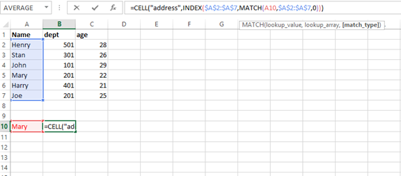
Example 2: From the above table use the data to look for text in column A and return the relative absolute cell reference.
Go to cell A10 and type Mary

On cell B10, type the formula =CELL("ADDRESS",INDEX(($A$2:$A$7,MATCH(A10,$A$2:$A$7,0)))

Press enter key

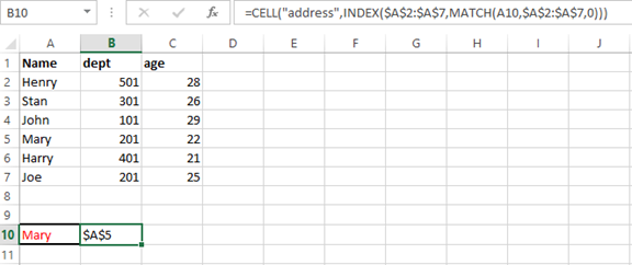
From the above example cell, B10 returns cell reference with the text Mary.
Cell A2:A7 is the column range with the lookup text, A10 is the lookup text.
The formula can only find the first relative cell address which matches the lookup text.
Example 3:
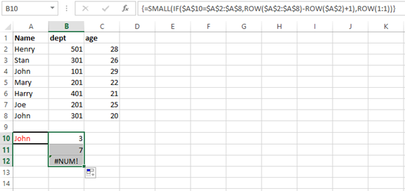
A formula to return the row number of the cell value in the table.
Look for an employee called John and return the cell address.
On cell B10 type the formula =SMALL(IF($A$10=$A$2:$A$8,ROW($A$2:$A$8)-ROW($A$2)+1),ROW(1:1)) and press Shift+ Ctrl+ Enter keys

Drag the Autofill handle down to copy the formula until #NUM! appears.

