In excel sheets we freeze columns, rows, or cells to make them visible all through the entire excel sheet even when we scroll from top to bottom. Excel sheets provide its users with the function or the tool to freeze rows, columns, cells, and panes
Freezing is the general activity of locking columns and rows in a given excel sheet so that when you happen to scroll top to down your rows or columns remain visible. We do freezing with the help of the freezing tool located under the view menu on the menu bar.
When data is on freeze function, it is made all visible throughout the entire sheet even when you scroll to the bottom cell of your data. This function helps the user keep a track of important data because it will always appear visible on the screen.
To do freezing is not a hard thing do, with the help of the following steps, you can freeze your work that is rows and columns at your convenient pace.
Step 1
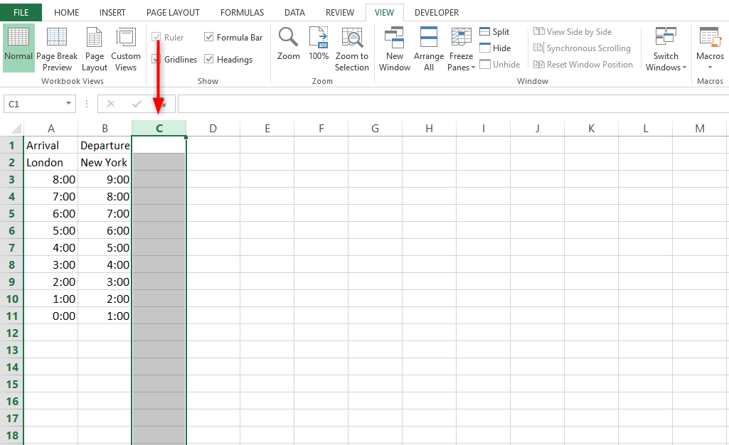
First of all, you will need to have the data set in an excel sheet that you would like to freeze the columns. If you do not have the data set to work on, open a blank excel sheet from Microsoft Excel on your laptop and insert some columns with data in them as in the case below.

Step 2
The second step is to select the columns you wish to lock. In this case, we are going to select two columns because they are the ones we are interested in at the moment. Note to freeze two columns you need to select the third column.

After you are done with the selection, go to the menu bar, and select on view. Under view, browse to find freeze panes. Click on freeze panes to reveal the list of options, select the first option which is freeze panes. This option will freeze or rather lock the two columns in a way that they will always remain visible even after scrolling down.

The sample excel sheet below explains the entire procedure in the picture form.

Consider data showing student scores. This dataset, therefore, contains student IDs, names, and their respective scores. Scrolling in excel from left to right moves everything. What if we wanted t to have the first two columns of ID and name to be visible regardless of how further right we scrolled? We can ensure this by freezing the said columns in excel. Here’s how;
Freeze 2 Columns Using Freeze Panes Option in Excel
Steps:
1. Count two columns from where the data begins then select the third column. In this case, select column C.

2. Hit View on the Excel ribbon then look for Freeze Panes > Freeze Panes

A gray vertical line appears between the second and third columns. This means that the first two columns (A and B) are frozen.

Apply Excel Split Option
Split functionality in excel is meant to break data into two distinct sets. This means you can navigate both sets of data by scrolling right or left on individual sets.
Steps:
1. Select column C.

2. On the excel ribbon, go to View, then Split.

3. You will realize that this cuts your worksheet into two datasets, independent with scroll areas.

Using Magic Freeze Button in Excel
Firstly, you need to add the magic freeze button from the Quick Access Toolbar. From here, we’ll use this button to freeze the first two columns.
Steps:
1. Click on the Customize Quick Access Toolbar icon (a small arrow pointing downwards) below or above the excel ribbon panel. Select the More Commands

2. On the resultant Excel Options window, choose Freeze Panes options under the Popular Commands box. Click on Add, and then OK.

3. The magic freeze button will then be added to the Quick Access Toolbar.

4. Repeat the same procedure from the freezing panes method.
5. Select column C and click Freeze Panes from the Magic Freeze button. This freezes the first two columns.

Use VBA Code
Steps:
1. Right-click on the sheet name on which data you want to freeze.
2. Click on the View Code option to bring up the VBA window.

3. Type the code below in the module window
Sub Freeze2Columns()
Columns("C:C").Select
ActiveWindow.FreezePanes = True
End Sub

4. Press the F5 key on the keyboard or the Run button to run the code.

5. The first two columns of the worksheet will freeze.
Simultaneously Freeze Rows and 2 Columns
You might want to diversify or decide at the same time to freeze columns and rows. There is a simpler way to simultaneously freeze the two columns and rows in excel. Here is how.
Steps:
1. Unlight in the previous methods where we highlighted an entire column. Here we only select a cell right to the column, and below the row, you want to freeze.
2. Then go to View> Freeze Panes > Freeze Panes.

You will see a gray line striking through horizontally and vertically indicating frozen columns and rows.
Things to Note
+ You cannot apply multiple free panes in a single excel worksheet.
+ You cannot use both Freeze Panes and Split options in an excel worksheet at the same time.
It is not possible to freeze a column located in the middle of the worksheet. This can be explained by the fact that no multiple freeze functionalities can be used in the same excel sheet at the same time.
You can freeze the first two columns in the Excel worksheet by using the keyboard shortcuts.
Press: Alt + W + F + F
Conclusion
You can give us feedback on how the article has been beneficial to you, and in case you got queries, don’t hesitate to contact us.
