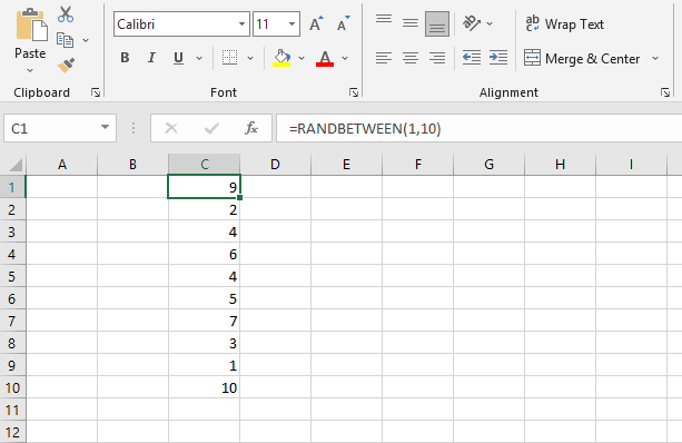
Random numbers are automated generated numbers that are displayed without an order. When working on a worksheet, the user may need to generate random numbers to perform various tasks. This is achievable due to the existence of two worksheet functions that are responsible for generating random numbers. They include The RAND function and the RANDBETWEEN function. In the RANDBETWEEN function, the random numbers generated may be the same, and therefore there is a high possibility of repeats in the number generated, whereas the RAND function is able to overcome this defect as it gives output without repetitions.
In this tutorial, we shall discuss the steps encountered when using the mentioned functions to generate random numbers.
Using RANDBETWEEN function
This function is of great importance when the user is generating numbers within a specified range. The user is able to input both the upper and lower number of ranges within its function. To effectively use this function to generate random numbers, the following super easy steps are used.
1. Open the excel
Double click the Excel app icon, which resembles a green with a white "X" on it. And then, open either a new document or an existing document on your device.
2. Select cell(s) to random input numbers
Click on the cell(s) where you want your random numbers to appear. If you are working on many cells, make sure you highlight all the cells before inserting the function.

3. Enter the function
In the formula bar, enter the function, =RANDBETWEEN (bottom, top). For example, if you want to generate random numbers between 1 and 10, then your upper value is ten, whereas 1 is the lower value.

4. Hold the CTRL key and press ENTER key
Once the function and the cell(s) are set, hold the control key and press the Enter key to generate a random number(s). These numbers will be automatically placed on each of the cell(s) that you had selected earlier.

Using RAND()
When the excel user wants to generate a random number that does not repeat, this is the best excel function to do this. To achieve this, the following steps are used:
1. Select cell(s) to random input numbers
Click on the cell(s) where you want your random numbers to appear just like it is in the previous method.
2. Enter the function
In the active cell, enter the function, =RAND (). And then, Hold the control button and press the Enter button. The numbers will be automatically be loaded on the selected cells.

However, this method generates numbers with decimal places. To convert the generated number to whole numbers, a RANK excel formula is used.
3. Converting random numbers to values
Firstly, write the RANK formulae on the active cell, =RANK.EQ (the indexes of cells that contain RAND () results) and then select the cell(s) that contain the result of the RAND function. By doing so, you will end up with whole numbers as random numbers.
