
Inactivating cell(s) in ms excel is pretty easy. Making the cell(s) inactive prevents the user from editing it, overwriting, or changing the content present on that particular cell. Through this feature, the data on the excel document is protected or locked. In Ms. Excel, the inactive is selected for all cells by default, and all the cells are automatically locked or inactivated. However, if you don't want to inactive all the cells, you can alternatively you can unlock all cells first and then inactive that specific cell and then protect the sheet.
If you experience a problem in inactivating the Ms. Excel cell(s), this article is specifically made for you. To make this feature familiar and easy to use for everyone, we shall discuss a method you can use to inactivate the cell in Ms. Excel. The methods use features present on the Ms. Excel application.
This method involves the following steps in disabling excel's cell(s):
1. Click on the excel icon to open the application. After that, open the document you want to edit. Otherwise, create a new document by inputting data on the provided cells.

2. Once you've opened the application and open the document you want to edit, select the cell(s) which you only want to make inactive.

3. Right-click on the selected cell(s) to access the side features of excel.

4. Scroll downwards and locate the "Format cell." Click on it to customize the selected cells. This feature is important in making the cells inactive.

5. On the new page displayed, locate the protection bar found on the screen's top-left side. Click on this bar.

6. Check if the locked box is checked. If not the case, click on the small box found on the left side of the word "Locked." Then click on it to ensure the highlighted cells are locked or inactivated.

Finally, click the "ok" button to confirm the changes.
7. After clicking the Ok button, then make the rules set to apply by activating the function protection sheet. Click on the review tab>>protect the sheet. On the protect sheet screen, a box is provided that allows the password that will be used to inactivate the cell(s). Click on the box and input your choice's password (optional as one can proceed without having to set a password).

8. Then, check the "select locked cells" if not checked. This is done by clicking on the small box found on the left side of the word "select locked cells." Finally, click the Ok button to inactivate the cells. You can go a step further and save your edit document and try to check if the feature applies.

‘Go To Special’ Feature to Lock A Group of Cells in Excel
You can use the Go To Special feature in Excel to pick all cells that fulfill a set of criteria easily. The feature is used to lock a group of cells.
Steps:
1. Select the cells with formulas. For example, D13 and E13 are selected.
2. Go to the Home tab on the ribbon.
3. Click on the Find & Select drop-down menu bar from the Editing group.

4. Select the Go To Special feature.

5. Select the Formulas from the Select list.
6. Click on the OK button to lock them.

7. Press the F4 key from your keyboard to lock the group of cells.
Using the Review Tab In Excel To Freeze A Group Of Cells
This feature includes features such as adding and deleting comments, protecting and unprotecting excel sheets/workbooks, and allowing users to follow changes in a multi-user excel workbook.
1. Select the whole data.
2. Go to the Review tab on the ribbon.
3. Select the Protected Sheet command under Protect group to open the Protect Sheet dialog box.

4. Save a password and click OK.

5. Confirm the password by typing the password again in the Reenter password to proceed type the box on the Confirm Password dialog.
6. Click on the OK button. A pop-up window appears.

7. Click ok to continue.
If you want to Unprotect the sheet, just click on the Unprotect Sheet. Type the password that you previously saved and click OK to view the locked cells.
Manually Lock A Group Of Cells From Ribbon
1. Select the cells that you want to lock.
2. Go to the Home tab.
3. Select Lock Cell from the Format drop-down menu, under the Cells category.
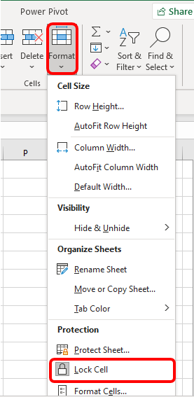
4. Click ok on the error shown up on the cells and select Lock Cells.
Lock a Group of Cells with Absolute References in Excel Formula
You can use absolute referencing to lock a group of cells. If you paste the formula someplace else in our worksheet or use the Fill Handle to copy the formula by utilizing absolute reference techniques to lock the cells, the cells existing inside the formula will not change to other relative locations. The ‘$' symbol in Excel stands for Absolute Reference.
1. Select the cell where you want to use the formula with absolute references.
2. Type the formula there and press Enter. The formula will calculate the total mark.
3. Drag the Fill Handle to copy the formula to lock the cells with absolute references.

Use the SUM function to sum the total sum number of marks.
To calculate the total normal price, type the formula in the respective cell and hit the Enter button.
=SUM($C$5:$C$13)

Also, you can calculate the total by typing the formula below in the respective cell and pressing Enter.
=SUM($E$5:$E$13)

The same will happen with any data that could follow with formulas in respective cells.
Freeze Group of Cells by Protecting Workbook
This method allows you to restrict which cells are utilized for entering data. Thus, it prevents other people to make changes to your spreadsheets or delete your worksheets.
Steps:
1. Select the sheet from which you want to lock a group of cells.
2. Go to the Review tab from the ribbon.
3. Select Protect Workbook under Protect category.

Using Excel VBA to Lock a Group of Cells in Excel
You can lock or protect your spreadsheets using VBA code. VBA is the most user-friendly and effective technique to automate Excel. Excel VBA enables advanced navigation and complicated execution.
1. Go to the Developer tab on the ribbon.

2. Click on Visual Basic or press Alt + F11 to open the Visual Basic Editor. You can also open the Visual Basic Editor by right-clicking on the sheet and selecting View Code.
3. Write down the VBA Code below;
VBASub LockCells()
Dim lckCell As Range
Dim lckRng As Range
ActiveSheet.Unprotect
Range("B4:E13").Locked = False
Set lckRng = ActiveSheet.Range("B4:E13")
For Each lckCell In lckRng.Cells
If lckCell.Value <> "" Then Cells.Locked = True
Next lckCell
ActiveSheet.Protect
End Sub Code

4. Run the code by pressing the F5 key or clicking the Run Sub button. The cell’s range B4:E13 is locked.
Through the above steps and procedures, anyone can comfortably make a cell inactive through the lock feature without any difficulty. Therefore, go ahead and create your document to try to make the cells inactive.