Formatting cells to be different from other cells makes them to stand out and get noticed.
Conditional formatting enables you to create rules that automatically change the cells formatting based on classified criteria or value of the cells.
Adding conditional formatting to your pivot table makes them look more attractive and have the "wow" factor. It also makes it easy to read the reports.
Pivot table is an important tool for analyzing and summarizing data.
Rules for applying conditional formatting in pivot tables can be modified based on user preferences.
This article will guide you on steps you can use to apply conditional formatting to your pivot table and create an appealing pivot report.
How to use conditional formatting.
1. Copy the table below

2. Create a pivot table from the above data.

3. Select a cell or range of cells in the values area
Select a cell where you want to add conditional formatting in the values area. If your pivot table has multiple fields in the value area then you can select the cells from the field you want to apply conditional formatting.

4. Apply conditional formatting to the cell
On the Home tab menu, choose conditional formatting. The dropdown arrow shows various options you can use to format your data.

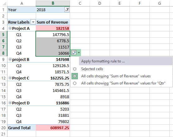
In this example, I will choose the top item rules then choose the top 10. I format the cells to get the top 2 cells with the highest value and change the color to Light Red fill and a text in dark red color.

Click ok.

5. Using the Formatting option Menu
You can click on the formatting option icon on your screen to apply more formatting to the fields in the values area.

Once you select the second option, you can see the cells highlighted in red including the grand total which has the highest value.
Conditional formatting for multiple fields

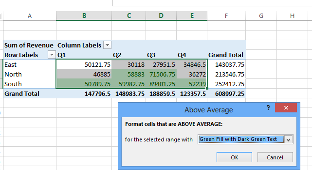
- From the pivot table, Select B5:E7 as shown above
- Go to the home tab and click conditional formatting
- Click on the top and bottom Rules and click above average
- In the open dialog box, select the formatting rules for your pivot table. And click ok.

The cells with above-average values are selected.
If you add more data to the source table, you need to refresh your pivot table so that the changes are also updated in your pivot table.
Right-click the pivot table and then click Refresh.
You can also insert bars in your Pivot table or insert icons.

