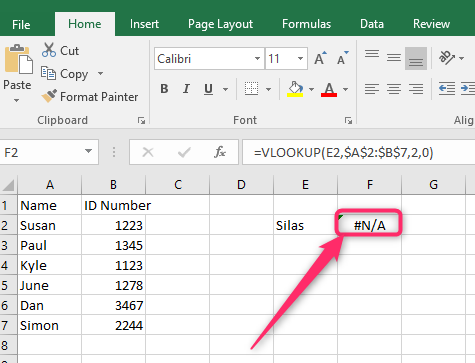
There are several types of errors that you can encounter while using the Excel application. #N/A error is one of the common errors one will likely encounter while using formulas in Excel. This error occurs when the formula used cannot find the referenced values. These errors make the data ugly for presentation. Thankfully, one can use the IFERROR function to eliminate this error. In this article, we shall discuss ways of using IFERROR and VLOOKUP functions to eliminate #N/A errors.
IFERROR Function Syntax
The IFEEROR function sets the returning value if the referenced cell returns an error value. To new users, the Function may be confusing. Here is the syntax of the Function:
=IFERROR(value, value_if_error)
Each part of the Function is clearly explained below:
=IFERROR( – This is how you should initialize the IFEEROR function in the formula bar.
Value- In this case, value refers to the cell reference or argument being checked for errors. When using the VLOOKUP with the IFERROR function, the VLOOKUP is the argument and value in this case.
Value_if_error – This is the value or phrase returned if the error is found in the referenced cell or argument.
To remove #N/A errors using the IFERROR with VLOOKUP
Here are the steps to follow:
1. Open the Excel application.
2. Double-click on the cell that contains the error. Copy the formula that returns the error. You will need it in the argument section of the IFERROR function.

3. Edit the formula that returns the error. Then, type the =IFERROR(Function.
4. Next, paste the VLOOKUP function that returns the error in the Value part of the Function. For example, =IFERROR(VLOOKUP(E2,$A$2:$B$7,2,0)
5. Then, type the Value_if_error that will remove the #N/A error. For example, =IFERROR(VLOOKUP(E2,$A$2:$B$7,2,0),"Not Found")

6. Finally, hit the Enter button.

Nesting IFERROR with the VLOOKUP function
Steps to follow:
1. Open the Excel application.
2. Double-click on the cell that contains the error. Copy the formula that returns the error. You will need it in the argument section of the IFERROR function.

3. Edit the formula that returns the error. Then, type the =IFERROR(Function.
4. Next, paste the VLOOKUP function that returns the error in the Value part of the Function. For example, =IFERROR(VLOOKUP(E2,$A$2:$B$7,2,0)
5. Then, add the IFERROR function to the formula. For example, =IFERROR(VLOOKUP(E2,$A$2:$B$7,2,0),IFERROR(VLOOKUP(E2,$A$2:$B$7,2,0),"Not Found"))

6. Finally, hit the Enter button.

To replace #N/A Error with a blank
Steps to follow:
1. Open the Excel application.
2. Double-click on the cell that contains the error.

3. Edit the formula that returns the error. Then, type the =IFERROR(Function.
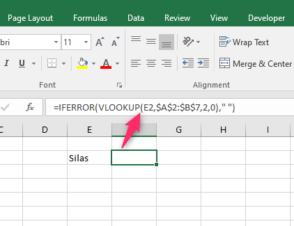
4. Next, paste the VLOOKUP function that returns the error in the Value part of the Function. For example, =IFERROR(VLOOKUP(E2,$A$2:$B$7,2,0)
5. Then, type the Value_if_error that will remove the #N/A error. In this case, we will leave the Value_If_error section blank. For example, =IFERROR(VLOOKUP(E2,$A$2:$B$7,2,0)," ")

6. Finally, hit the Enter button.

