
Pivot Table is a useful tool for checking Excel's distinct and unique values. A pivot table is used for a dataset with duplicate values. This article will discuss ways of counting Unique values in Excel.
To count Unique Values with Helper Column
Steps:
1. Open the Excel application.
2. Enter the dataset in the empty cells. Alternatively, open an existing Excel document with the dataset you wish to convert to a Pivot Table.
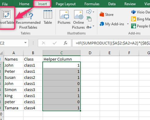
3. Create another column beside your dataset, and name it Helper Column. In the Helper Column, enter this formula: =IF (SUMPRODUCT(($A$2:$A2=A2)*($B$2:$B2=B2))>1,0,1) and hit the Enter button.

4. Drag the formula to other cells down the column.

5. Click on the Insert tab on the Ribbon. The Insert tab is located on the far-left side of the Ribbon and in the Tables section.
6. Then, click on the PivotTable button. In the Create PivotTable dialogue box, ensure the selected cells are captured in the Table/Range section.
7. Next, toggle on the New Worksheet if you want the Pivot Tables to be displayed on a new worksheet. If you need the Pivot table to appear on the same Worksheet, toggle on the Existing Worksheet. If you choose the Existing Worksheet, click on the Location section and add the cell references where the Pivot table will be displayed.
8. Then, click the OK button. The selected dataset will automatically be converted to a Pivot Table.

9. In the PivotTable Fields pane, check the checkboxes of one column and the Helper column.

10. That is. The Pivot table with unique values will be shown.

To count Unique Values with Data Model
Steps:
1. Open the Excel application.
2. Enter the dataset in the empty cells.
3. Highlight the cells that have the dataset. To highlight cells, press the CTRL + A keys or click on the Left mouse and move the cursor along the dataset you wish to highlight.

4. Click on the Insert tab on the Ribbon. The Insert tab is located on the far-left side of the Ribbon and in the Tables section.
5. Then, click on the PivotTable button. In the Create PivotTable dialogue box, ensure the selected cells are captured in the Table/Range section.

6. Next, toggle on the New Worksheet or Existing Worksheet.
7. Check the "Add this data to the Data Model" checkbox.
8. Finally, hit the OK button.

9. Right-click on the added Pivot Table and choose the Value Field Setting option from the side-view menu.

10. In the Value field Settings, locate the "Summarize value field by" section. From this section, choose the Count option, and click the OK button. That is all you need to do.
