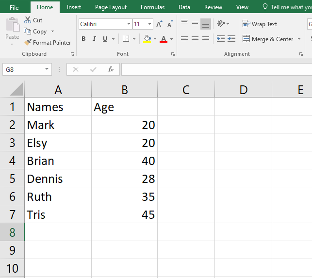
A worksheet is a collection of cells. There are a lot of operations that can be conducted on the worksheet. Some of the common ones include:
a) Renaming a worksheet
Procedure:
1. Launch Excel.
2. Ensure you are on the active worksheet which is to be renamed.

3. Right-click on the Worksheet tab. A menu will pop up

4. Select "Rename"
5. The worksheet tab will get a blinking cursor suggesting you edit the name.

6. Type in your Name of choice. Then press Enter.

7. The worksheet tab will now assume the new name.
b) Copying a worksheet
An existing worksheet can be duplicated with all its content.
Procedure:
1. Launch the Excel project.
2. Open a worksheet that contains some data in it

3. Right-click on the worksheet tab. A shortcut menu will pop up

4. Select the "Move or Copy" option from the menu

5. A move or copy Dialog will be displayed. Select the workbook under the "To book".

6. You can change the arrangement of the new worksheet with respect to the existing ones using the Before sheet.
7. Check the create copy Box Then Click OK

C) Positioning worksheets
Existing worksheets can be repositioned or arranged accordingly. To reposition a worksheet:
Procedure:
1. Right-click on one of the worksheet tabs.

2. Select "Move or Copy"
3. Under the Before Sheet: Select "move to end" or any of the existing worksheets.

4." Move to end for example positions the current worksheet to the end.
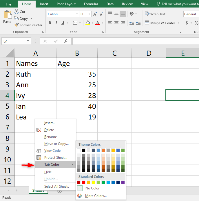
d) Changing the worksheet tab color
1. Right-click the worksheet tab

2. Select tab color from menu options

3. Select your color from the list of colors that pops up.
e) Inserting a new worksheet
To insert a new blank worksheet:
1. Right-click on the tab

2. Select Insert.
3. Click on the Worksheet and press OK

4. A new blank worksheet will get launched.
f) Applying Filters to worksheets
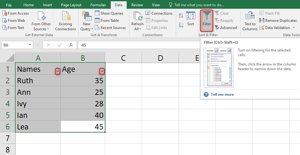
Filtering enables us to extract crucial information from what we have. This is usually very helpful especially for large sets of data. To apply the filter:
Procedure:
1. Select the data you intend to apply the filter on. Ensure that column heads are highlighted too.

2. Navigate to the Data tab from Excels Ribbon

3. Click on Filter. Dropdown arrows are then displayed

4. Click on the Items dropdown. Type R and click OK. Note that only Items whose names start with an F are highlighted.

g) Ranking in worksheets
One can rank a given field using the Rank function. For example, we can rank the costs of different items to find the most expensive ones in that order.
Procedure:
1. Create a new Column.
2. Add a label/heading e.g. Oldest

3. Add a rank formula while inside the first empty cell just under the Header.
Syntax:
=RANK(B2,$B$2:$B$6,1)

4. Press Enter.
5. Drag and drop along the Rank column starting with the first cell into which you type the formula. Cost ranking will be done using the individual oldest column.

NB: B2 is used as the starting point for the rank. The dollar sign in the reference indicates that it's a relative reference and the Formula should thus change depending on the position of the order. The last part, 1, refers to the order of rank which means ascending order while Zero, on the other hand, implies rank in descending order.
