Vlookup is a very useful Excel Function. Basically, what it does is ‘Look-up’ or searches for a value or text specified in a table (array) and returns a value or text from another column, also specified. One disadvantage of this Excel Function is that the value or text being looked up must be in the first column of the table.
Without many theoretical explanations, let us go into how to make use of this Function with examples.
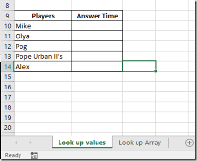
In this tutorial, we will be considering a situation where the Lookup table is in another spreadsheet in the same Workbook. See the below images.
We are going to fill Cells B10 to B14 with Answer Time values gotten from the Lookup Array sheet. Basically, to fill cell B10 with the accurate time it took “Mike” to answer the questions, we need a function that will go into the Look up Array Sheet and look for “Mike” under the Players column, which happens to be the first column in this table, and return “6.87”. The best formula for this kind of task is the Vlookup function because the column which contains the Look-up values can be found on the first column of the table.
VLOOUP format
The format in which the Vlookup has to be written is as follows:
VLOOKUP (lookup_value, table_array, col_index_num, [range_lookup])
1.) Lookup_value: It is the value being looked up. It can be a text (the text must be in quoted commas), number, or a cell reference.
2.) table_array: It is the table that contains the value being looked up. The column containing the lookup value must be the first column in this array.
3.) col_index_num: The is the column number in the above table_array which contains the value to be returned.
4.) [range_lookup]: Here is where you specify whether you are looking for an Exact match (FALSE) or an approximate match (TRUE). This field is not compulsory. The default option is FALSE
Here we go:
– Click on cell B10 in the lookup Value sheet, which is the first empty cell in the Answer Time column
– Click Insert Function
– Type Vlookup in the Search for a function: box
– Click Go
– Click OK
– Click in the Lookup_value field and select cell A10
– Click in the Table_array field and select the Table in the Lookup Array sheet
– Type 2 in the Col_index_num field. This denotes Answer Time is in the 2nd column in the Array
– Type FALSE in Range_lookup field
– Click OK
– You can then do an auto-fill to apply the formula to other cells in the column. To do this, with Cell B10 selected, place your mouse at the bottom right corner of the cell where there is a tiny square. At this point, your cursor would turn to a Plus sign, then double click or click and drag up until Cell B14.
You will notice there is a #N/A error. This is because “Alex” is not one of the names in the Lookup Array.


