In this tutorial, we will be discussing how to create a basic line graph on Microsoft Excel 2016.
Line graphs are generally used to show trends of a series of data points. It is typically used to show the behavior of a metric / data set over time (week, months year…).
Here are the steps to follow in creating a Line Chart:
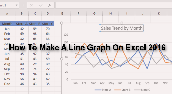
1. Highlight the data set you want to see in a Line Chart. See the example below, Range A2:D14 has been selected.

2. Go to the Insert Tab and Click on the Line Chart drop-down button  in the Charts group and select the first option from the drop-down menu.

3. You will then see the Line Chart on the sheet. You can resize the chart by clicking and dragging from the 4 corners of the chart. As you can see, the blue line represents Store A, the Orange line represents Store B and the grey line represents Store C.

4. To change the Chart Title, click on the "Chart Title" and Type "Sales Trend by Month" and press Enter

For more options to format the graph, double click anywhere on the chart area, a panel will appear on the right-hand side of the sheet. You can play around with the different options available.
Sometimes, you might want to have a combination of Lines and Columns on the graph, to do this, with the graph selected:
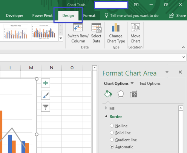
A. Go to the Design Tab and click on Change Chart Type. It is located on the far-right-hand side after Select Data. See the image below.

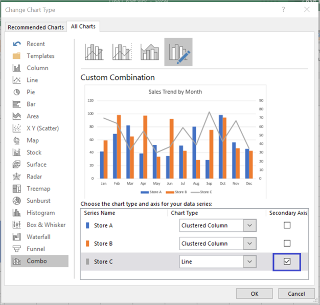
B. In this example, we'd like to represent the data for Store A and Store B as Clustered Columns. In the "Choose the chart type and axis for your data series:" section, change the chart type for Store A and Store B as shown below.

C. For Store C, you could also check the Secondary Axis box, so it does not share the same axis with Store A and Store B because they are Clustered columns and Store C is the only data point represented by a Line graph

D. Click OK.
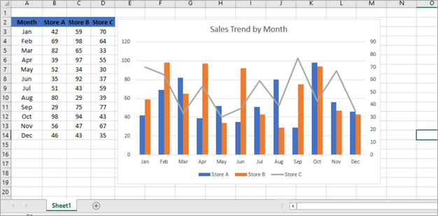
See the below image for the final chart. As you can see it is a combo of Clustered Columns and Line Graphs.

