
Globally, people have grown to use excel sheets in their day-to-day activities to perform general and specific functions. Excel sheets provide users with numerous capabilities and functionalities. People use excel to record data on findings, to do graphs, and also charts. All these functionalities are geared to a neat representation of data.
Excel sheets provide its users with the function or the tool to freeze rows, columns, and panes. The act of locking columns and rows in an excel sheet so that when you scroll top to down your rows or columns remain visible is what is referred to as freezing.
As said earlier, when data is on freeze function, it is made all visible throughout the entire sheet even when you scroll to the bottom cell of your data. This function helps the user keep a track of important data because it will always appear visible on the screen.
To do freezing of rows, there are a couple of steps that are followed, these steps may include;
Step 1
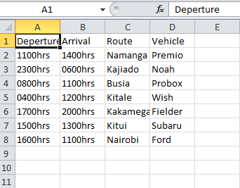
The first step is to come up with the data that we wish to deal with. On your device, whether a laptop or a computer, open a blank excel sheet and feed it some general data of your choice.
Step 2
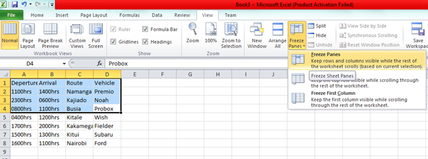
Now that we have our excel sheet prepared, the next step will be to freeze the top 4 rows.
We are going to highlight the first four rows because they are the ones we wish to lock, after that we go to the menu bar and click on view. Under view, search for freeze panes and click on it. A list of options appears to select the option of freeze panes which is the first option.
You will realize that after following the above steps, the top four cells will remain visible even after scrolling to the bottom of the excel sheet. That is how basically freeze panes function does to the excel sheets rows, columns, and cells. Take a look at the image of the screenshot below.
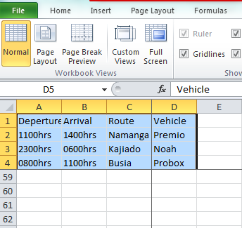
The four cells will remain that way until you execute the unfreeze function.