
When working with excel sheets, you may have similar data that you are working with and which are in different excel sheets. Such data can be pulled from one of the sheets to another. This will save time in writing data in the columns or rows again.
To pull data from one excel sheet to another is the process of taking the data, be it in a column or a row, to another excel sheet. Once we pull values from another sheet, which is commonly done, we can save on time taken which we would otherwise keep in inserting the values in columns or rows.
Errors are minimized because while inserting the data all over again; you may omit some values, which will cause issues in the data set.
We have several procedures to follow to pull data from other sheets; the steps involved include the ones below;
Using Enter and Save
First, open a new excel sheet; in sheet 1, insert data as in the case below.

Leave the column with the estate as the header empty.
In sheet 2, enter the data as follows and save the excel sheet as "sheet2"

Using VLOOKUP Function
Having our sheets set with data values, we will now try and see if we can pull the values from sheet 2 to sheet 1. We have a function that we are going to use; the VLOOKUP function. This function will help us pull data values from sheet 2 to sheet 1. You can also pull data values from any other sheet you wish.
The formula that we will write on the formula bar of sheet 1 will be; = VLOOKUP (B3, 'Sheet 2'! $B$3: $C$6, 2, 0). This formula on column B values will keep changing because B3 is only the first cell.

The formula will be able to pull the values of column C from sheet 2 upon clicking on the enter button, as in the case below.

The values will automatically be displayed in column C with the header Estate in both sheet 1 and sheet 1.
Using Advanced Filter in Excel
The Advanced Filter is among the easiest ways to use if you want to pull data from another sheet in Excel. For example, you can use it to pull data of customers and their payment details from one sheet and record it in the new worksheet. In this case, you can follow these simple steps:
1. Open the second spreadsheet and click on the Data button.

2. Select the Advanced option from the Sort and Filter commands.

3. A new dialogue box will show up. Select the Copy to another location option under the Action menu.

4. Next, fill in the List range box from the original worksheet. You can also click on the up-facing arrow to select the range directly.
5. Click on the Criteria range and select the data based on the criteria you want.
6. Finish by selecting the cell where you want the extracted data to appear and click the OK button.

If you wanted to pull data of customers who paid using their cards, you get your result showing only those who paid with cards in your preferred range of cells.
Using Combined INDEX And MATCH Functions
You can also combine INDEX and MATCH functions to pull data from one sheet to another based on your preferred criteria. The combination is among the powerful Excel hacks; hence, you can use it to extract customers' payment details such as amount or payment mode. When using the combination, the MATCH function locates the matching value from the array of another sheet, while the INDEX function returns that value from the list. To pull data on customers' amounts, you can follow these steps:
1. On a new sheet, select the cell you want to pull from the source sheet. For example, you can select cell D5, which has the customers’ value.
2. Write the following formula in the cell:
=INDEX('INDEX & MATCH Functions'!B5:E5,MATCH($B$5,'INDEX & MATCH Functions'!$B$4:$E$4,0))

3. Press the Enter key, and you will see the extracted amount in the new cell.
4. You can now use the cursor or Fill Handle to drag the formula down the column. This will automatically pull data from the source sheet to the new column.

Using the HLOOKUP Function
The HLOOKUP is a unique function to look up data horizontally and bring back the value. For instance, you can use it to pull out customers' payment history into another worksheet through the following steps:
1. On the new sheet, select the cell with the dataset you want to pull out. For example, you can select cell E5.
2. Write the following formula in the cell and press the Enter button.
=HLOOKUP($B$5,'HLOOKUP Function'!$B$4:$E$8,Sheet4!D5+1,0)

3. You can now use the cursor or Fill Handle to drag the formula down the cells.
4. The function will pull out all the customers' payment history from the source sheet and return the data to the new sheet.

Using Cell References
Of all the methods, using relevant cell references is the simplest way to pull data from one Excel sheet to another. Here, you can use these steps:
1. Select the cell where you want the extracted data to appear.

2. Type the equal sign (=) followed by the name of the sheet you want to pull data from. Enclose the sheet name in single quote marks if the name of the sheet is more than one word. Type the '!' sign followed by the cell reference of the cell you to pull data from.
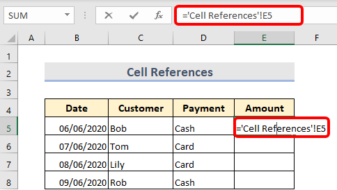
3. Press the Enter button, and the data from your source sheet will appear in the new cell.
4. You can now drag the Fill Handle (+) icon down the column to pull data from other remaining cells.
