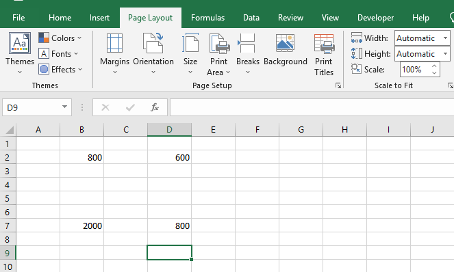
At times we work with large worksheets in an Excel workbook. It becomes a dreaded issue when you want to combine all your data, as most people automatically think it will mean retyping all that text. Now you can breathe a sigh of relief because, when you are working with data in Excel, it is easier to merge data entries in different cells, rows, and even columns.
There are different ways of achieving this using the Excel formula. Let us look at some of the methods.
Method A: Use Concatenate function to combine cells
The Concatenate function in Excel means to combine or join together. It is the same function as that of Google sheets. The function is simple and easy when looking to combine multiple cells into one.
It is a powerful Excel tool and a go-to method as it can help limit time wasted on repetitive data entry. Here is a guide on what you have to do.
1. Open your spreadsheet.
2. Select your preferred cell in the worksheet that you want to combine cells.

3. Type CONCATENATE. Remember, like all excel formulas, start by the sign = before you write Concatenate. Next, use the opening and closing parenthesis, and type in the cell locations, which tell the function cells to combine. For example, =CONCATENATE(A2, B2, C2) or =CONCATENATE(AA, BB, CC)

4. Adjust the formula to include any needed punctuation marks like separators, and quotation marks to add spaces, commas, or other texts. For example, =CONCATENATE(A2, ", ", B2, " ", C2)
5. Close the formula when done, and press Enter.

Method B: Combine data with the Ampersand symbol (&)
1. Select your preferred cell

2. Type = sign and select the first cell you want to combine. For example, B2

3. Type quotation marks with a space enclosed. For example, B2&."

4. Select the second cell you want to combine and press ENTER. Your formula will end up looking like this =A2&" "&B2&" &C2

Method C: Use the Text join Function to combine cells
This method is mainly used in Excel 365 and later versions as it is a new function.
1. Open your spreadsheet.
2. Select the cell to put the combined data.

3. Type =TEXTJOIN

4. Select the cells you want to combine into one cell.
5. Remember to include separators. Your function will end up like this =TEXTJOIN(", ", TRUE,A2:C2)

NOTE;
- When you want to update data in one of the original cells, any changes made in uncombined cells will be reflected automatically in the combined cell.
- These methods are not limited to only three cells. The formula works with large amounts of data, columns, and rows you might want to combine.
- Use the option "Paste as text" in case you want to copy and paste the data into another spreadsheet or worksheet. It will prevent data changes.
Conclusion
From the article above, we get to know different methods of combining multiple cells, in our case 3 into one cell. Choosing either one of them will lead to the same results and help reduce duplication.
