Excel is the best tool to use for database analysis. It refers to a combination of rows and columns, and these rows and columns are used for storing our data as records. The excel rows and columns are further divided into smaller cells where the record data is inputted. Excel records can be converted into a table to form an excel database, and this makes the life of a regular excel user easier.
When creating an excel database, you need to carefully design the excel worksheet to have proper info in the database format.
1. Open the excel worksheet
Before accessing any feature on excel, you have to launch an excel application and create a new worksheet where you will add your data. Click on the excel option and tap the "New" button.


2. Entering the data
When entering the data in the worksheet, each cell is used to input each data of the database. Firstly, label the heading properly of your data.
After
the headers of the data table are clear, you can start entering data on the cells below the respective column headings. However, carefulness should be observed when entering data to ensure you don't leave a single row empty. Similarly, you cannot have an empty column between the data. Therefore, fill in the data carefully.

3. Select the inputted data
Once all the data is inputted, highlight all the cells that contain the information to be converted to a database. Click the left mouse at the beginning of the data and then scroll down until all the required data are highlighted.

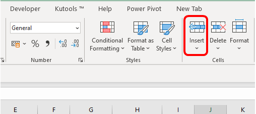
4. Click the "Insert" button
On the ribbon bar, locate and click on the insert button. Then, click the table button located on the leftmost side of the insert section. Alternatively, you can use excel's shortcut to access the table feature. By selecting the data and then pressing Ctrl+T.

Here you need to make sure the header check box is checked and the data range shown selected properly. If the table header is not checked, you can activate it by clicking on the small box located on the left. Once everything is completely set, click the "ok" button.


5. Customize the database table
Since we've created a table, we have the database ready now, and it can be used for further references. When you enter the data after the last column, it will expand automatically. Excel is fitted with features that enable users to edit and make the table more appealing. These features are found under the table design tab. For example, if you wish to give your table a proper name, click the Table name tab on the Design tab, edit it and input the proper name of your table and then save by clicking anywhere on the worksheet screen.

Go ahead and click the excel tools button, and then click the save button to save your database.
Create Database in Excel
Before getting into database creation, Let's first learn something about databases in excel.
You cannot at any instance enter data and leave a row between two entries empty. Here’s an illustration.

Some cells can be empty in a database and it is completely legal. Leaving a complete row empty, however, is illegal.
Furthermore, it is not a good practice when you leave a full column empty.

The reason you should never leave an empty row or column is that whenever Excel encounters such a gap, it treats the data after such rows or columns as a new set of database. Therefore, the functions you deploy would not be able to filter on the disconnected part.
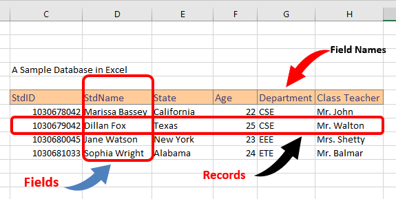
Rows are called Records, while columns are known as Fields. Headings on the columns are known as Field names.

The following are steps to creating a database in Excel;
i). Start by creating a data spreadsheet in excel.
Ensure that the columns are properly headed. Columns are labeled alphabetically while rows are named numerically.
1. Open the Excel Sheet on your PC. Click on one cell to insert header names. The Tab button on your screen helps you to navigate from one row to a column. Once through, the cursor will take you to the next row or column.
2. Enter data or import from other sources. For instance, go to the Home tab, find the Cells segment and click on the Insert dropdown button. You cannot leave any row empty.

For data importation, look for the Data tab, look for Get Data and choose the destination of your data.

ii). Convert your data into a table.
Data should be converted into a table. Click on any cell with information and select Insert>Table. Ensure data is in the correct format. Once done, data will be directly incorporated, and click Ok on the pop-up table.

How to arrange data in your spreadsheet using excel.
1. Spreadsheet database using Simple Horizontal Gray cells.
For long, this method has been useful to excel users, and it is segmented into two forms. Horizontal and vertical modes.
The horizontal database on the spreadsheet is dated in one row. Dates on the column use monthly buckets. However, they could use any time required. The codes column uses general ledger accounts. Gray rows and columns are the most common features of simple cells.
2. Simple spreadsheet database vertical style.
One column of data is comprised of several fields. In this case, data is shown vertically.
Names are easy to allocate in this format. In a classic excel, select Insert, go to Name, and Create.
In a new excel, select formulas, proceed to Defined names, and create from the selection.

3. Excel tables
Typically, after setting tables, more columns and rows, are named automatically.
Look out for the following.
- Data Arranged
- Headers and Data
To confirm;
Select Insert
Go to Tables on the Create Table Dialog
Make sure that the table has headers and press OK
Excel will automatically name the tables i.e Table 1, Table 2 e.t.c
4. Tabular layout for pivot tables
Pivot tables have different benefits like exploring data that is relatable in excel. It returns sorted, sliced, and summarized data in spreadsheets.
Setting up a pivot database table to look like an excel table
Insert a pivot table using these simple steps:
- Go to the Data Set and click any single
- Go to Tables group, then Insert tab and click Pivot Table. Excel will select the data for you.
- Click OK on the pop-up table.

The pivot table Fields pane will appear that will show the total amount of exported data. Drag the following: product field to rows area, amount field to value area, and country field to filters area.

- Sort the table by accessing the cell inside the sum amount and clicking on it.
- Right-click on sort and sort from right to left.
