How to find the area under the graph in Excel

Area Under graph is a common concept in integral and data science classes. Did you know you can find the area under the graph using the Excel Tool? There is no in-built tool or function for calculating the area under the graph in Excel. However, some workarounds can be used to determine the area of the graph. The workarounds are not difficult as they are straightforward and involve tools present in Excel. In this post, we will discuss the common methods of calculating area in Excel.

Table of Contents

Using Formula and SUM function

The area under the graph is like a trapezoid; therefore, the formula for calculating trapezoid can be used together with the SUM function to calculate the area. Here is the formula for calculating a trapezoid:

A = (a+b)/2 * h

Where:

A= is the area

a= this is the base of one side

b= this is the base length of the other side

h= is the height of the trapezoid

Let us now discuss steps to calculate the area using this method:

1. Open the Excel application.

2. Open the Workbook that contains the worksheet with your dataset. Add your dataset to the sheet if you're using a new workbook.

3. Highlight the dataset you wish to convert to a graph. Then, click the Insert tab on the Ribbon.

4. Then click the Insert tab on the Ribbon. In the Chart section, click the Insert Scatter or Bubble Chart drop-down button. From the menu, choose the Scatter with a straight-line graph.

5. On clicking, a scatter graph is inserted into your active chart. Add another column in your dataset and name it "Area." Under this column, type this formula =(B2+B3)/2*(A3-A2) on the first cell in the Area column.

Note: This formula depends on the location of your dataset.

6. Hit the Enter button, and then drag the formula to the second-last cell in the Area column.

7. Locate another cell and type the SUM function. That is =SUM (

Then select all the cells in the Area column and hit the Enter button. For Example, SUM(A2:A7)

Using the Trend line Tool

Steps to follow:

1. Open the Excel application.

2. Open the Workbook that contains the worksheet with your dataset. Add your dataset to the sheet if you're using a new workbook.

3. Highlight the dataset you wish to convert to a graph. Then, click the Insert tab on the Ribbon.

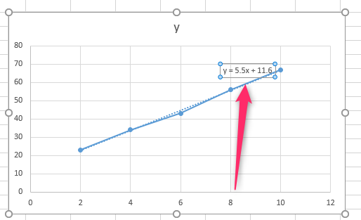
5. On clicking, a scatter graph is inserted into your active chart. Click on the Plus Sign icon, hover the cursor over the Trend Line option and choose the More Options button.