
Sometimes, you may need to highlight the entire row based on a particular cell value. If you are working on a large dataset, you need to know how to highlight the entire row based on cell value quickly. This article will discuss ways of highlighting rows based on the partial match.
Using Conditional Formatting Tool
a) Using the SEARCH formula to highlight the row
Here are the steps to follow:
1. Open the Excel application.
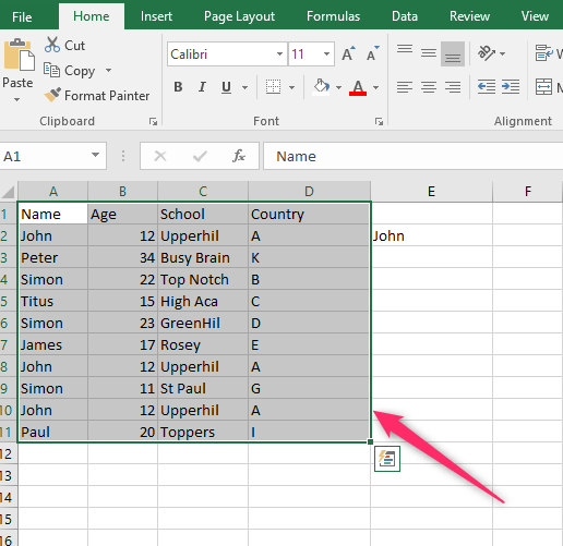
2. Open the existing document that contains the dataset you wish to search for data. Then, create a helper cell containing the value you want to search.

3. Highlight the dataset on which you wish to search data or apply the conditional formatting.

4. Click on the Home tab on the ribbon, and locate the Styles section.
5. Click the Conditional Formatting drop-down button. From the drop-down menu, click the New Rule button.

6. A New Formatting Rule dialogue box will open. In the dialogue box, choose the "Use a formula to determine which cell to format" option.
7. In the "Format values where this formula is true:" section, type the following formula: =AND($E$2<>" ",ISNUMBER(SEARCH($E$2,$A2)))

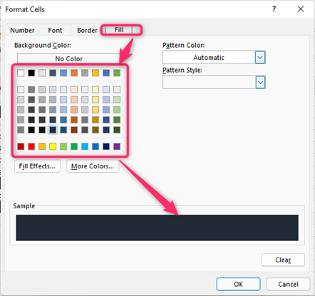
8. Click on the Format button. In the Format Cells dialogue box, click on the Fill tab. Choose the background color you want to apply from the Background Color.

9. Click OK to save the changes. That is all you need to do.

b) Using the Text criterion
Steps:
1. Open the Excel application.
2. Open the existing document that contains the dataset you wish to search for data.
3. Highlight the dataset you wish to search data or apply the conditional formatting.
4. Click on the Home tab on the ribbon, and locate the Styles section.
5. Click the Conditional Formatting drop-down button. From the drop-down menu, click the New Rule button.

6. A New Formatting Rule dialogue box will open. In the dialogue box, choose the "Use a formula to determine which cell to format" option.
7. In the "Format values where this formula is true:" section, type the following formula:=$A2= "John"

8. Click on the Format button. In the Format Cells dialogue box, click on the Fill tab. Choose the background color you want to apply from the Background Color.
9. Click OK to save the changes. That is all you need to do.

c) Using the number criterion
Steps:
1. Open the Excel application.
2. Highlight the dataset you wish to search data or apply the conditional formatting.

3. Click on the Home tab on the ribbon, and locate the Styles section.
4. Click the Conditional Formatting drop-down button. From the drop-down menu, click the New Rule button.

5. A New Formatting Rule dialogue box will open. In the dialogue box, choose the "Use a formula to determine which cell to format" option.
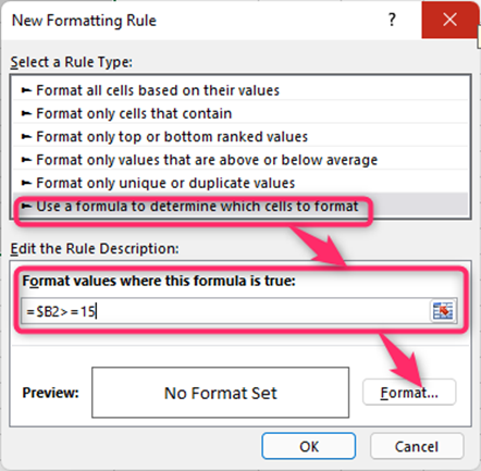
6. In the "Format values where this formula is true:" section, type the following formula:=$B2>=15
7. Click on the Format button. In the Format Cells dialogue box, click on the Fill tab. Choose the background color you want to apply from the Background Color.

8. Click OK to save the changes. That is all you need to do.